%matplotlib inline

Analyze Visium fluorescence data

This tutorial shows how to apply Squidpy image analysis features for the analysis of Visium data.

For a tutorial using Visium data that includes the graph analysis functions, have a look at Analyze Visium H&E data. The dataset used here consists of a Visium slide of a coronal section of the mouse brain. The original dataset is publicly available at the 10x genomics dataset portal <https://support.10xgenomics.com/spatial-gene-expression/datasets>_ . Here, we provide a pre-processed dataset, with pre-annotated clusters, in anndata.AnnData format and the tissue image in squidpy.im.ImageContainer format.

A couple of notes on pre-processing:

- The pre-processing pipeline is the same as the one shown in the original
  `Scanpy tutorial <https://scanpy-tutorials.readthedocs.io/en/latest/spatial/basic-analysis.html>`_ .
- The cluster annotation was performed using several resources, such as the
  `Allen Brain Atlas <https://mouse.brain-map.org/experiment/thumbnails/100048576?image_type=atlas>`_ ,
  the `Mouse Brain gene expression atlas <http://mousebrain.org/>`_
  from the Linnarson lab and this recent pre-print {cite}`linnarson2020`.

Import packages & data

To run the notebook locally, create a conda environment as conda env create -f environment.yml using this environment.yml <https://github.com/scverse/squidpy_notebooks/blob/main/environment.yml>_.

import pandas as pd

import matplotlib.pyplot as plt

import anndata as ad
import scanpy as sc
import squidpy as sq

sc.logging.print_header()
print(f"squidpy=={sq.__version__}")

# load the pre-processed dataset
img = sq.datasets.visium_fluo_image_crop()
adata = sq.datasets.visium_fluo_adata_crop()

scanpy==1.9.2 anndata==0.8.0 umap==0.5.3 numpy==1.23.5 scipy==1.9.3 pandas==1.5.1 scikit-learn==1.1.3 statsmodels==0.13.2 python-igraph==0.10.2 pynndescent==0.5.7
squidpy==1.2.3

100%|██████████| 303M/303M [00:44<00:00, 7.19MB/s] 
100%|██████████| 65.5M/65.5M [00:09<00:00, 7.20MB/s]

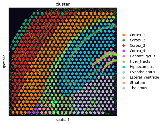
First, let’s visualize the cluster annotation in the spatial context with squidpy.pl.spatial_scatter().

As you can see, this dataset is a smaller crop of the whole brain section. We provide this crop to make the execution time of this tutorial a bit shorter.

sq.pl.spatial_scatter(adata, color="cluster")

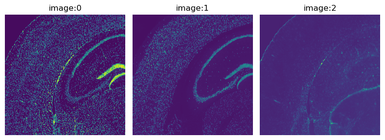
The fluorescence image provided with this dataset has three channels: DAPI (specific to DNA), anti-NEUN (specific to neurons), anti-GFAP (specific to Glial cells). We can directly visualize the channels with the method squidpy.im.ImageContainer.show().

img.show(channelwise=True)

Visium datasets contain high-resolution images of the tissue. Using the function squidpy.im.calculate_image_features() you can calculate image features for each Visium spot and create a obs x features matrix in adata that can then be analyzed together with the obs x gene gene expression matrix.

By extracting image features we are aiming to get both similar and complementary information to the gene expression values. Similar information is for example present in the case of a tissue with two different cell types whose morphology is different. Such cell type information is then contained in both the gene expression values and the tissue image features. Complementary or additional information is present in the fact that we can use a nucleus segmentation to count cells and add features summarizing the immediate spatial neighborhood of a spot.

Squidpy contains several feature extractors and a flexible pipeline of calculating features of different scales and sizes. There are several detailed examples of how to use squidpy.im.calculate_image_features(). Extract image features provides a good starting point for learning more.

Here, we will extract summary, histogram, segmentation, and texture features. To provide more context and allow the calculation of multi-scale features, we will additionally calculate summary and histogram features at different crop sizes and scales.

Image segmentation

To calculate segmentation features, we first need to segment the tissue image using squidpy.im.segment(). But even before that, it’s best practice to pre-process the image by e.g. smoothing it using in squidpy.im.process(). We will then use the DAPI channel of the fluorescence image (channel_id s= 0). Please refer to Cell-segmentation for fluorescence images for more details on how to calculate a segmented image.

sq.im.process(
    img=img,
    layer="image",
    method="smooth",
)

sq.im.segment(img=img, layer="image_smooth", method="watershed", channel=0, chunks=1000)

# plot the resulting segmentation
fig, ax = plt.subplots(1, 2)
img_crop = img.crop_corner(2000, 2000, size=500)
img_crop.show(layer="image", channel=0, ax=ax[0])
img_crop.show(
    layer="segmented_watershed",
    channel=0,
    ax=ax[1],
)

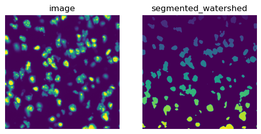
The result of squidpy.im.segment() is saved in img['segmented_watershed'] by default. It is a label image where each segmented object is annotated with a different integer number.

Segmentation features

We can now use the segmentation to calculate segmentation features. These include morphological features of the segmented objects and channel-wise image intensities beneath the segmentation mask. In particular, we can count the segmented objects within each Visium spot to get an approximation of the number of cells. In addition, we can calculate the mean intensity of each fluorescence channel within the segmented objects. Depending on the fluorescence channels, this can give us e.g., an estimation of the cell type. For more details on how the segmentation features, you can have a look at the docs of squidpy.im.calculate_image_features() or the example at Extract segmentation features.

# define image layer to use for segmentation
features_kwargs = {"segmentation": {"label_layer": "segmented_watershed"}}
# calculate segmentation features
sq.im.calculate_image_features(
    adata,
    img,
    features="segmentation",
    layer="image",
    key_added="features_segmentation",
    n_jobs=1,
    features_kwargs=features_kwargs,
)
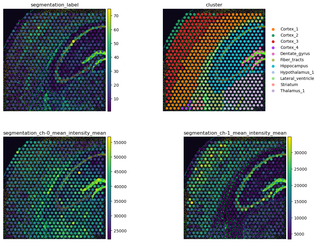
# plot results and compare with gene-space clustering
sq.pl.spatial_scatter(
    sq.pl.extract(adata, "features_segmentation"),
    color=[
        "segmentation_label",
        "cluster",
        "segmentation_ch-0_mean_intensity_mean",
        "segmentation_ch-1_mean_intensity_mean",
    ],
    frameon=False,
    ncols=2,
)

100%|██████████| 704/704 [01:35<00:00,  7.40/s]

Above, we made use of squidpy.pl.extract(), a method to extract all features in a given adata.obsm['{key}'] and temporarily save them to anndata.AnnData.obs. Such method is particularly useful for plotting purpose, as shown above.

The number of cells per Visium spot provides an interesting view of the data that can enhance the characterization of gene-space clusters. We can see that the cell-rich pyramidal layer of the Hippocampus has more cells than the surrounding areas (upper left). This fine-grained view of the Hippocampus is not visible in the gene clusters where the Hippocampus is one cluster only.

The per-channel intensities plotted in the second row show us that the areas labeled with Cortex_1 and Cortex_3 have a higher intensity of channel 1, anti-NEUN (lower left). This means that these areas have more neurons that the remaining areas in this crop. In addition, cluster Fiber_tracts and lateral ventricles seems to be enriched with Glial cells, seen by the larger mean intensities of channel 2, anti-GFAP, in these areas (lower right).

Extract and cluster features

Now we will calculate summary, histogram, and texture features. These features provide a useful compressed summary of the tissue image. For more information on these features, refer to:

• Extract summary features.

• Extract histogram features.

• Extract texture features.

# define different feature calculation combinations
params = {
    # all features, corresponding only to tissue underneath spot
    "features_orig": {
        "features": ["summary", "texture", "histogram"],
        "scale": 1.0,
        "mask_circle": True,
    },
    # summary and histogram features with a bit more context, original resolution
    "features_context": {"features": ["summary", "histogram"], "scale": 1.0},
    # summary and histogram features with more context and at lower resolution
    "features_lowres": {"features": ["summary", "histogram"], "scale": 0.25},
}

for feature_name, cur_params in params.items():
    # features will be saved in `adata.obsm[feature_name]`
    sq.im.calculate_image_features(
        adata, img, layer="image", key_added=feature_name, n_jobs=1, **cur_params
    )

# combine features in one dataframe
adata.obsm["features"] = pd.concat(
    [adata.obsm[f] for f in params.keys()], axis="columns"
)

# make sure that we have no duplicated feature names in the combined table
adata.obsm["features"].columns = ad.utils.make_index_unique(
    adata.obsm["features"].columns
)

100%|██████████| 704/704 [02:34<00:00,  4.56/s]
100%|██████████| 704/704 [01:32<00:00,  7.62/s]
100%|██████████| 704/704 [01:40<00:00,  6.97/s]

We can use the extracted image features to compute a new cluster annotation. This could be useful to gain insights in similarities across spots based on image morphology.

For this, we first define a helper function to cluster features.

def cluster_features(features: pd.DataFrame, like=None):
    """
    Calculate leiden clustering of features.

    Specify filter of features using `like`.
    """
    # filter features
    if like is not None:
        features = features.filter(like=like)
    # create temporary adata to calculate the clustering
    adata = ad.AnnData(features)
    # important - feature values are not scaled, so need to scale them before PCA
    sc.pp.scale(adata)
    # calculate leiden clustering
    sc.pp.pca(adata, n_comps=min(10, features.shape[1] - 1))
    sc.pp.neighbors(adata)
    sc.tl.leiden(adata)

    return adata.obs["leiden"]

Then, we calculate feature clusters using different features and compare them to gene clusters:

adata.obs["features_summary_cluster"] = cluster_features(
    adata.obsm["features"], like="summary"
)
adata.obs["features_histogram_cluster"] = cluster_features(
    adata.obsm["features"], like="histogram"
)
adata.obs["features_texture_cluster"] = cluster_features(
    adata.obsm["features"], like="texture"
)

sc.set_figure_params(facecolor="white", figsize=(8, 8))
sq.pl.spatial_scatter(
    adata,
    color=[
        "features_summary_cluster",
        "features_histogram_cluster",
        "features_texture_cluster",
        "cluster",
    ],
    ncols=3,
)

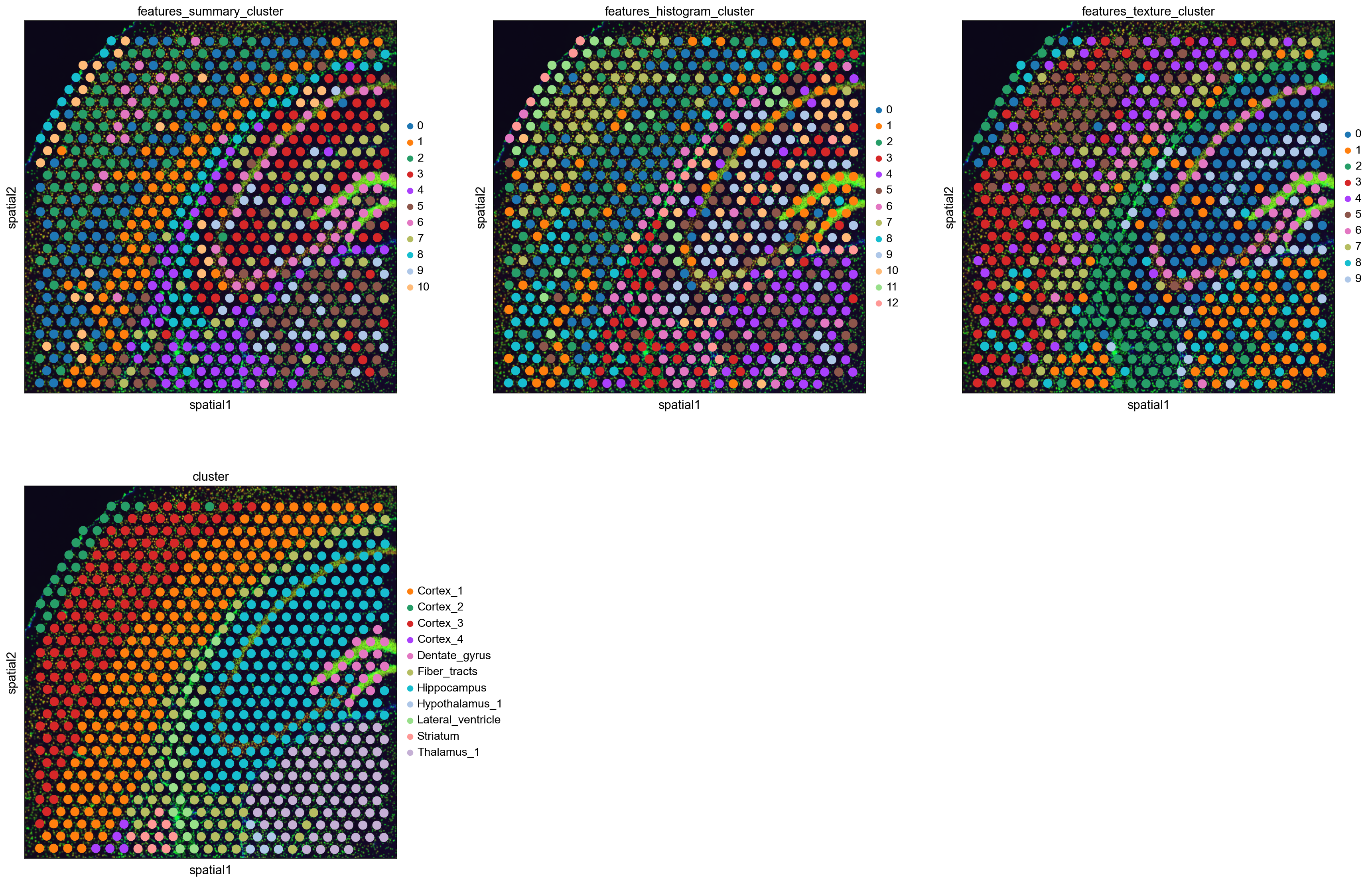
Like the gene-space clusters (bottom middle), the feature space clusters are also spatially coherent.

The feature clusters of the different feature extractors are quite diverse, but all of them reflect the structure of the Hippocampus by assigning different clusters to the different structural areas. This is a higher level of detail than the gene-space clustering provides with only one cluster for the Hippocampus.

The feature clusters also show the layered structure of the cortex, but again subdividing it in more clusters than the gene-space clustering. It might be possible to re-cluster the gene expression counts with a higher resolution to also get more fine-grained clusters, but nevertheless the image features seem to provide additional supporting information to the gene-space clusters.