%matplotlib inline
Extract texture features
This example shows how to extract texture features from the tissue image.
Textures features give give a measure of how the image intensity at
different distances and angles varies by calculating a grey-level
co-occurrence matrix
(GLCM). The GLCM
includes the number of times that grey-level \(j\) occurs at a distance
\(d\) and at an angle \(\\theta\) from grey-level \(i\). From this data,
different features (props) are calculated. See also
skimage.feature.greycomatrix.
Texture features are calculated by using features = 'texture', which
calls squidpy.im.ImageContainer.features_texture(). In addition to
feature_name and channels, we can also specify the following
features_kwargs:
distances- distances that are taken into account for finding repeating patterns.
angles- range on which values are binned. Default is the whole image range.
props- texture features that are extracted from the GLCM.
See also
See {doc}`compute_features` for general usage
of {func}`squidpy.im.calculate_image_features`.
import squidpy as sq
Let’s load the fluorescence Visium dataset and calculate texture
features with default features_kwargs.
Note that for texture features it may make sense to compute them over a
larger crop size to include more context, e.g., spot_scale = 2 or
spit_scale = 4 which will extract crops with double or four times the
radius than the original Visium spot size. For more details on the image
cropping, See Crop images with ImageContainer.
# get spatial dataset including high-resolution tissue image
img = sq.datasets.visium_fluo_image_crop()
adata = sq.datasets.visium_fluo_adata_crop()

# calculate texture features and save in key "texture_features"
sq.im.calculate_image_features(
    adata,
    img,
    features="texture",
    key_added="texture_features",
    spot_scale=2,
    show_progress_bar=False,
)
The result is stored in anndata.AnnData.obsm\ ['texture_features'].
adata.obsm["texture_features"].head()
| texture_ch-0_contrast_dist-1_angle-0.00 | texture_ch-0_contrast_dist-1_angle-0.79 | texture_ch-0_contrast_dist-1_angle-1.57 | texture_ch-0_contrast_dist-1_angle-2.36 | texture_ch-0_dissimilarity_dist-1_angle-0.00 | texture_ch-0_dissimilarity_dist-1_angle-0.79 | texture_ch-0_dissimilarity_dist-1_angle-1.57 | texture_ch-0_dissimilarity_dist-1_angle-2.36 | texture_ch-0_homogeneity_dist-1_angle-0.00 | texture_ch-0_homogeneity_dist-1_angle-0.79 | ... | texture_ch-2_homogeneity_dist-1_angle-1.57 | texture_ch-2_homogeneity_dist-1_angle-2.36 | texture_ch-2_correlation_dist-1_angle-0.00 | texture_ch-2_correlation_dist-1_angle-0.79 | texture_ch-2_correlation_dist-1_angle-1.57 | texture_ch-2_correlation_dist-1_angle-2.36 | texture_ch-2_ASM_dist-1_angle-0.00 | texture_ch-2_ASM_dist-1_angle-0.79 | texture_ch-2_ASM_dist-1_angle-1.57 | texture_ch-2_ASM_dist-1_angle-2.36 | |
|---|---|---|---|---|---|---|---|---|---|---|---|---|---|---|---|---|---|---|---|---|---|
| AAACGAGACGGTTGAT-1 | 42.783204 | 79.464035 | 41.904014 | 82.624826 | 1.983783 | 2.753093 | 1.973759 | 2.743151 | 0.753973 | 0.725217 | ... | 0.570987 | 0.504941 | 0.883396 | 0.787901 | 0.872758 | 0.790485 | 0.040632 | 0.035577 | 0.041006 | 0.035397 |
| AAAGGGATGTAGCAAG-1 | 82.756940 | 144.883230 | 76.546612 | 159.714604 | 3.349644 | 4.369327 | 3.171514 | 4.603538 | 0.692667 | 0.666414 | ... | 0.538010 | 0.466651 | 0.938821 | 0.914061 | 0.947862 | 0.887927 | 0.016620 | 0.013672 | 0.016786 | 0.013555 |
| AAATGGCATGTCTTGT-1 | 27.093979 | 48.276535 | 23.560334 | 49.362415 | 2.416785 | 3.209199 | 2.249740 | 3.271754 | 0.565910 | 0.525931 | ... | 0.571515 | 0.503682 | 0.878716 | 0.781444 | 0.873200 | 0.786576 | 0.033804 | 0.028822 | 0.034247 | 0.028759 |
| AAATGGTCAATGTGCC-1 | 24.198313 | 36.550901 | 18.040215 | 46.083141 | 2.222673 | 2.732854 | 1.925904 | 3.103483 | 0.645956 | 0.621034 | ... | 0.578051 | 0.511233 | 0.988060 | 0.979815 | 0.987566 | 0.979121 | 0.016216 | 0.013678 | 0.016297 | 0.013659 |
| AAATTAACGGGTAGCT-1 | 21.413928 | 39.826111 | 23.691475 | 47.908006 | 1.281552 | 1.779400 | 1.349581 | 1.883277 | 0.821503 | 0.798561 | ... | 0.577136 | 0.507679 | 0.954380 | 0.926691 | 0.954430 | 0.922658 | 0.026097 | 0.022120 | 0.026564 | 0.022041 |
5 rows × 60 columns
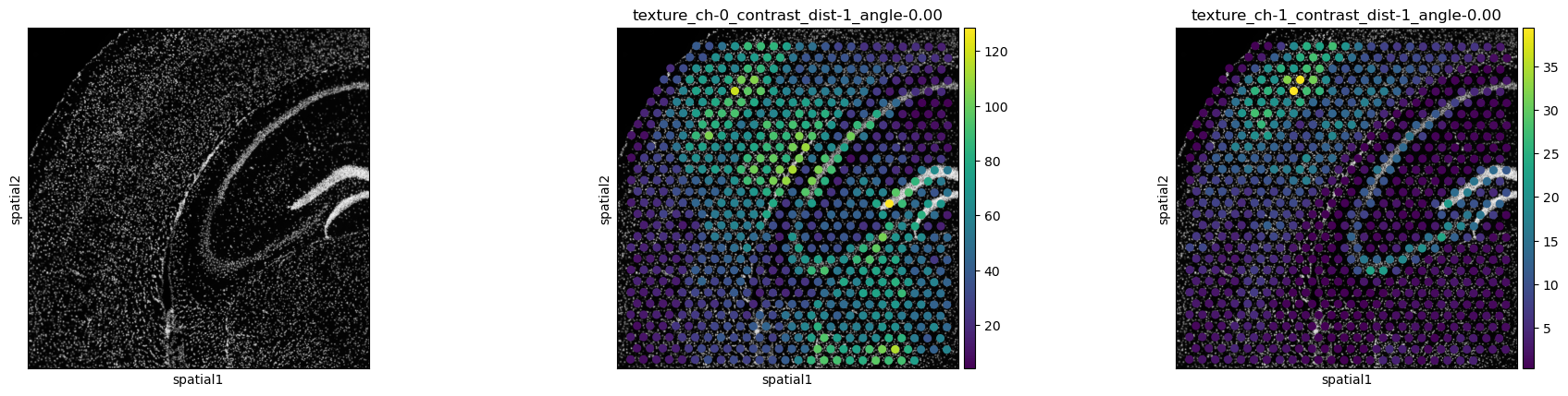
Use squidpy.pl.extract to plot the texture features on the tissue
image or have a look at napari-spatialdata for interactive visualization. Here, we show the contrast feature for
channels 0 and 1. The two stains, DAPI in channel 0, and GFAP in channel
1 show different regions of high contrast.
sq.pl.spatial_scatter(
    sq.pl.extract(adata, "texture_features"),
    color=[
        None,
        "texture_ch-0_contrast_dist-1_angle-0.00",
        "texture_ch-1_contrast_dist-1_angle-0.00",
    ],
    img_cmap="gray",
)