%matplotlib inline
Analyze 4i data
This tutorial shows how to apply Squidpy for the analysis of 4i data.
The data used here was obtained from [Gut et al., 2018].
We provide a pre-processed subset of the data, in anndata.AnnData format.
For details on how it was pre-processed, please refer to the original paper.
Import packages & data
To run the notebook locally, create a conda environment as conda env create -f environment.yml using this
environment.yml <https://github.com/scverse/squidpy_notebooks/blob/main/environment.yml>_.
import squidpy as sq

print(f"squidpy=={sq.__version__}")

# load the pre-processed dataset
adata = sq.datasets.four_i()
squidpy==1.2.2
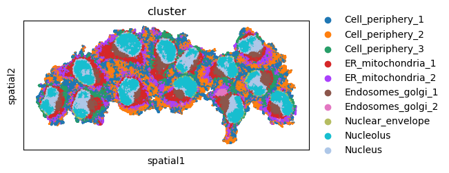
First, let’s visualize cluster annotation in spatial context
with squidpy.pl.spatial_scatter().
sq.pl.spatial_scatter(adata, shape=None, color="cluster", size=1)
WARNING: Please specify a valid `library_id` or set it permanently in `adata.uns['spatial']`
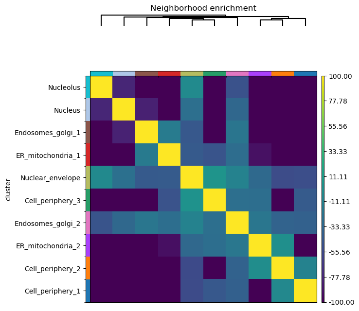
Neighborhood enrichment analysis
Similar to other spatial data, we can investigate spatial organization of clusters
in a quantitative way, by computing a neighborhood enrichment score.
You can compute such score with the following function: squidpy.gr.nhood_enrichment().
In short, it’s an enrichment score on spatial proximity of clusters:
if spots belonging to two different clusters are often close to each other,
then they will have a high score and can be defined as being enriched.
On the other hand, if they are far apart, the score will be low
and they can be defined as depleted.
This score is based on a permutation-based test, and you can set
the number of permutations with the n_perms argument (default is 1000).
Since the function works on a connectivity matrix, we need to compute that as well.
This can be done with squidpy.gr.spatial_neighbors().
Please see Building spatial neighbors graph for more details
of how this function works.
Finally, we’ll directly visualize the results with squidpy.pl.nhood_enrichment().
We’ll add a dendrogram to the heatmap computed with linkage method ward.
sq.gr.spatial_neighbors(adata, coord_type="generic")
sq.gr.nhood_enrichment(adata, cluster_key="cluster")
sq.pl.nhood_enrichment(adata, cluster_key="cluster", method="ward", vmin=-100, vmax=100)
100%|██████████| 1000/1000 [00:21<00:00, 45.75/s]
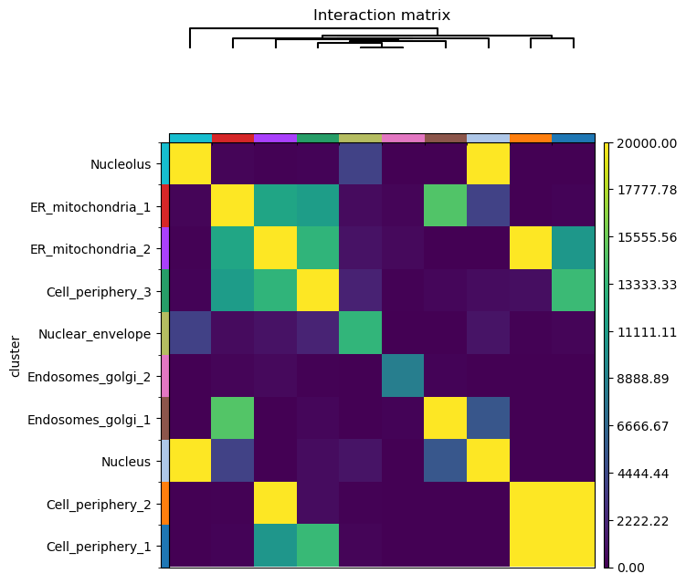
A similar analysis can be performed with squidpy.gr.interaction_matrix().
The function computes the number of shared edges in the neighbor graph between clusters.
Please see Compute interaction matrix for more details
of how this function works.
sq.gr.interaction_matrix(adata, cluster_key="cluster")
sq.pl.interaction_matrix(adata, cluster_key="cluster", method="ward", vmax=20000)
Additional analyses to gain quantitative understanding of spatial patterning of sub-cellular observations are:
Compute Ripley’s statistics for Ripley’s statistics.
Compute co-occurrence probability for co-occurrence score.
Spatially variable genes with spatial autocorrelation statistics
With Squidpy we can investigate spatial variability of gene expression.
This is an example of a function that only supports 2D data.
squidpy.gr.spatial_autocorr() conveniently wraps two
spatial autocorrelation statistics: Moran’s I and Geary’s C.
They provide a score on the degree of spatial variability of gene expression.
The statistic as well as the p-value are computed for each gene, and FDR correction
is performed. For the purpose of this tutorial, let’s compute the Moran’s I score.
See Compute Moran’s I score for more details.
adata.var_names_make_unique()
sq.gr.spatial_autocorr(adata, mode="moran")
adata.uns["moranI"].head(10)
| I | pval_norm | var_norm | pval_norm_fdr_bh | |
|---|---|---|---|---|
| Yap/Taz | 0.972975 | 0.0 | 0.000001 | 0.0 |
| CRT | 0.958505 | 0.0 | 0.000001 | 0.0 |
| TUBA1A | 0.939577 | 0.0 | 0.000001 | 0.0 |
| NUPS | 0.915073 | 0.0 | 0.000001 | 0.0 |
| TFRC | 0.895786 | 0.0 | 0.000001 | 0.0 |
| HSP60 | 0.889395 | 0.0 | 0.000001 | 0.0 |
| Actin | 0.879217 | 0.0 | 0.000001 | 0.0 |
| CTNNB1 | 0.876393 | 0.0 | 0.000001 | 0.0 |
| Climp63 | 0.873853 | 0.0 | 0.000001 | 0.0 |
| VINC | 0.862522 | 0.0 | 0.000001 | 0.0 |
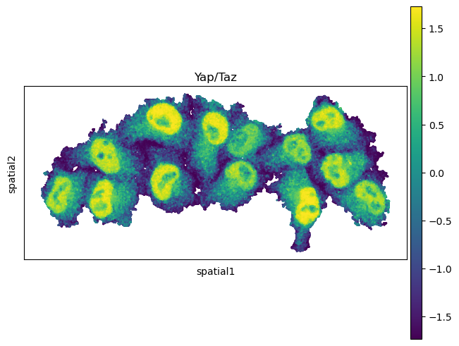
The results are stored in adata.uns['moranI'] and we can visualize selected genes
with squidpy.pl.spatial_scatter().
sq.pl.spatial_scatter(adata, shape=None, color="Yap/Taz", size=1)
WARNING: Please specify a valid `library_id` or set it permanently in `adata.uns['spatial']`