%matplotlib inline
Extract segmentation features
This example shows how to extract segmentation features from the tissue image.
Features extracted from a nucleus segmentation range from the number of
nuclei per image, over nuclei shapes and sizes, to the intensity of the
input channels within the segmented objects. They are very interpretable
features and provide valuable additional information. Segmentation
features are calculated by using features = 'segmentation', which
calls squidpy.im.ImageContainer.features_segmentation().
In addition to feature_name and channels we can specify the
following features_kwargs:
label_layer- name of label image layer inimg.props- segmentation features that are calculated. See [properties]{.title-ref} inskimage.measure.regionprops_table.
See also
Cell-segmentation for fluorescence images for more details on calculating a cell-segmentation.
Extract image features for the general usage of
squidpy.im.calculate_image_features().
import matplotlib.pyplot as plt

import squidpy as sq
First, let’s load the fluorescence Visium dataset.
img = sq.datasets.visium_fluo_image_crop()
adata = sq.datasets.visium_fluo_adata_crop()
Before calculating segmentation features, we need to first calculate a
segmentation using squidpy.im.segment.
sq.im.segment(
    img=img,
    layer="image",
    layer_added="segmented_watershed",
    method="watershed",
    channel=0,
)
Now we can calculate segmentation features. Here, we will calculate the following features:
number of nuclei
label.mean area of nuclei
area.mean intensity of channels 1 (anti-NEUN) and 2 (anti-GFAP) within nuclei
mean_intensity.
We use mask_cicle = True to ensure that we are only extracting
features from the tissue underneath each Visium spot. For more details
on the image cropping, see
examples_image_compute_crops.
sq.im.calculate_image_features(
    adata,
    img,
    layer="image",
    features="segmentation",
    key_added="segmentation_features",
    features_kwargs={
        "segmentation": {
            "label_layer": "segmented_watershed",
            "props": ["label", "area", "mean_intensity"],
            "channels": [1, 2],
        }
    },
    mask_circle=True,
)
The result is stored in anndata.AnnData.obsm\ ['segmentation_features'].
adata.obsm["segmentation_features"].head()
| segmentation_label | segmentation_area_mean | segmentation_area_std | segmentation_ch-1_mean_intensity_mean | segmentation_ch-1_mean_intensity_std | segmentation_ch-2_mean_intensity_mean | segmentation_ch-2_mean_intensity_std | |
|---|---|---|---|---|---|---|---|
| AAACGAGACGGTTGAT-1 | 17 | 174.764706 | 291.276810 | 5604.069561 | 3100.506862 | 8997.290710 | 177.888882 |
| AAAGGGATGTAGCAAG-1 | 14 | 100.785714 | 80.946348 | 5034.146353 | 1625.737796 | 10376.489346 | 564.254124 |
| AAATGGCATGTCTTGT-1 | 16 | 132.000000 | 147.241723 | 11527.768307 | 12227.308457 | 7725.282284 | 947.987907 |
| AAATGGTCAATGTGCC-1 | 9 | 243.000000 | 132.341310 | 3581.244911 | 46.124320 | 9664.505991 | 1331.259644 |
| AAATTAACGGGTAGCT-1 | 7 | 229.142857 | 203.573383 | 9038.077440 | 8707.493743 | 10922.808071 | 3631.149215 |
Use squidpy.pl.extract to plot the texture features on the tissue
image or have a look at napari-spatialdata. Here, we show all calculated segmentation
features.
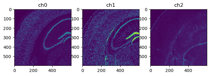
# show all channels (using low-res image contained in adata to save memory)
fig, axes = plt.subplots(1, 3, figsize=(8, 4))
for i, ax in enumerate(axes):
    ax.imshow(
        adata.uns["spatial"]["V1_Adult_Mouse_Brain_Coronal_Section_2"]["images"][
            "hires"
        ][:, :, i]
    )
    ax.set_title(f"ch{i}")

# plot segmentation features
sq.pl.spatial_scatter(
    sq.pl.extract(adata, "segmentation_features"),
    color=[
        "segmentation_label",
        "segmentation_area_mean",
        "segmentation_ch-1_mean_intensity_mean",
        "segmentation_ch-2_mean_intensity_mean",
    ],
    img_cmap="gray",
    ncols=2,
)
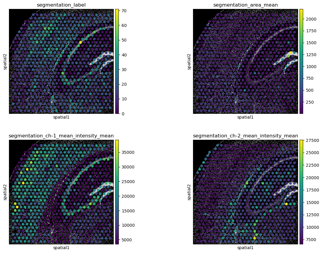
[segmentation_label]{.title-ref} shows the number of nuclei per spot and [segmentation_area_mean]{.title-ref} the mean are of nuclei per spot. The remaining two plots show the mean intensity of channels 1 and 2 per spot. As the stains for channels 1 and 2 are specific to Neurons and Glial cells, respectively, these features show us Neuron and Glial cell dense areas.