%matplotlib inline
Extract image features
This example shows the computation of spot-wise features from Visium images.
Visium datasets contain high-resolution images of the tissue in addition
to the spatial gene expression measurements per spot (obs). In this
notebook, we extract features for each spot from an image using
squidpy.im.calculate_image_features and create a obs x features
matrix that can be analyzed together with the obs x genes spatial
gene expression matrix.
See also
We provide different feature extractors that are described in more
detail in the following examples:
See Extract summary features on how to calculate summary statistics of each color channel.
See Extract texture features on how to calculate texture features based on repeating patterns.
See Extract histogram features on how to calculate color histogram features.
See Extract segmentation features on how to calculate number and size of objects from a binary segmentation layer.
See Extract custom features on how to calculate custom features by providing any feature extraction function.
import numpy as np

import seaborn as sns

import squidpy as sq

# get spatial dataset including high-resolution tissue image
img = sq.datasets.visium_hne_image_crop()
adata = sq.datasets.visium_hne_adata_crop()
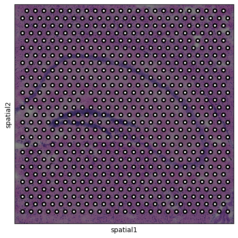
The high-resolution tissue image is contained in img['image'], and the
spot locations coordinates are stored in anndata.AnnData.obsm\ ['spatial'].
We can plot the spots overlayed on a lower-resolution version of the tissue
image contained in adata.
np.set_printoptions(threshold=10)
print(img)
print(adata.obsm["spatial"])

sq.pl.spatial_scatter(adata, outline=True, size=0.3)
ImageContainer[shape=(3527, 3527), layers=['image']]
[[1575   98]
 [2538 1774]
 [1850   98]
 ...
 [2263 1534]
 [2401 1055]
 [2676 1774]]
Using this information, we can now extract features from the tissue
underneath each spot by calling squidpy.im.calculate_image_features.
This function takes both adata and img as input, and will write the
resulting obs x features matrix to anndata.AnnData.obsm\ [<key>]. It contains
several arguments to modify its behavior. With these arguments you can:
specify the image used for feature calculation using
layer.specify the type of features that should be calculated using
featuresandfeatures_kwargs.specify how the crops used for feature calculation look like using
kwargs.specify parallelization options using
n_jobs,backend, andshow_progress_bar.specify how the data is returned using
key_addedandcopy.
Let us first calculate summary features and save the result in
adata.obsm['features'].
sq.im.calculate_image_features(
    adata, img, features="summary", key_added="features", show_progress_bar=False
)

# show the calculated features
adata.obsm["features"].head()
| summary_ch-0_quantile-0.9 | summary_ch-0_quantile-0.5 | summary_ch-0_quantile-0.1 | summary_ch-0_mean | summary_ch-0_std | summary_ch-1_quantile-0.9 | summary_ch-1_quantile-0.5 | summary_ch-1_quantile-0.1 | summary_ch-1_mean | summary_ch-1_std | summary_ch-2_quantile-0.9 | summary_ch-2_quantile-0.5 | summary_ch-2_quantile-0.1 | summary_ch-2_mean | summary_ch-2_std | |
|---|---|---|---|---|---|---|---|---|---|---|---|---|---|---|---|
| AAAGACCCAAGTCGCG-1 | 140.0 | 112.0 | 78.0 | 110.332029 | 24.126489 | 108.0 | 80.0 | 53.0 | 80.129908 | 21.863844 | 140.0 | 115.0 | 90.0 | 115.145057 | 19.554108 |
| AAAGGGATGTAGCAAG-1 | 144.0 | 114.0 | 90.0 | 115.557253 | 21.279808 | 107.0 | 77.0 | 56.0 | 79.957329 | 20.546552 | 142.0 | 111.0 | 88.0 | 113.362959 | 21.422890 |
| AAAGTCACTGATGTAA-1 | 139.0 | 115.0 | 84.0 | 112.740563 | 22.550223 | 121.0 | 94.0 | 66.0 | 93.735134 | 22.459672 | 141.0 | 118.0 | 93.0 | 117.298447 | 19.089482 |
| AAATGGCATGTCTTGT-1 | 138.0 | 109.0 | 74.0 | 107.372175 | 24.896688 | 101.0 | 71.0 | 45.0 | 72.320288 | 21.589912 | 142.0 | 111.0 | 85.0 | 112.642091 | 21.896309 |
| AAATGGTCAATGTGCC-1 | 146.0 | 113.0 | 84.0 | 113.296553 | 24.740431 | 112.0 | 77.0 | 53.0 | 80.073602 | 22.858352 | 144.0 | 113.0 | 89.0 | 115.193915 | 20.901613 |
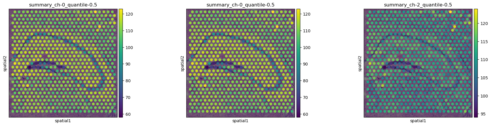
To visualize the features, we can use squidpy.pl.extract to plot the
texture features on the tissue image.
Here, we plot the median values of all channels ([summary_ch-0_quantile-0.5]{.title-ref}, [summary_ch-0_quantile-0.5]{.title-ref}, and [summary_ch-2_quantile-0.5]{.title-ref}).
sq.pl.spatial_scatter(
    sq.pl.extract(adata, "features"),
    color=[
        "summary_ch-0_quantile-0.5",
        "summary_ch-0_quantile-0.5",
        "summary_ch-2_quantile-0.5",
    ],
)
Specify crop appearance
Features are extracted from image crops that capture the Visium spots
(see also examples_image_compute_crops). By default,
the crops have the same size as the spot, are not scaled and square. We
can use the mask_circle argument to mask a circle and ensure that only
tissue underneath the round Visium spots is taken into account to
compute the features. Further, we can set scale and spot_scale
arguments to change how the crops are generated. For more details on the
crop computation, see also
examples_image_compute_crops.
Use
mask_circle = True, scale = 1, spot_scale = 1, if you would like to get features that are calculated only from tissue in a Visium spot.Use
scale = X, with [X < 1]{.title-ref}, if you would like to downscale the crop before extracting the features.Use
spot_scale = X, with [X > 1]{.title-ref}, if you want to extract crops that are X-times the size of the Visium spot.
Let us extract masked and scaled features and compare them.
We subset adata to the first 50 spots to make the computation of
features fast. Skip this step if you want to calculate features from all
spots.
adata_sml = adata[:50].copy()

# calculate default features
sq.im.calculate_image_features(
    adata_sml,
    img,
    features=["summary", "texture", "histogram"],
    key_added="features",
    show_progress_bar=False,
)
# calculate features with masking
sq.im.calculate_image_features(
    adata_sml,
    img,
    features=["summary", "texture", "histogram"],
    key_added="features_masked",
    mask_circle=True,
    show_progress_bar=False,
)
# calculate features with scaling and larger context
sq.im.calculate_image_features(
    adata_sml,
    img,
    features=["summary", "texture", "histogram"],
    key_added="features_scaled",
    mask_circle=True,
    spot_scale=2,
    scale=0.5,
    show_progress_bar=False,
)

# plot distribution of median for different cropping options
_ = sns.displot(
    {
        "features": adata_sml.obsm["features"]["summary_ch-0_quantile-0.5"],
        "features_masked": adata_sml.obsm["features_masked"][
            "summary_ch-0_quantile-0.5"
        ],
        "features_scaled": adata_sml.obsm["features_scaled"][
            "summary_ch-0_quantile-0.5"
        ],
    },
    kind="kde",
)
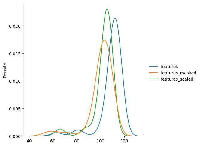
The masked features have lower median values, because the area outside the circle is masked with zeros.
Parallelization
Speeding up the feature extraction is easy. Just set the n_jobs flag
to the number of jobs that should be used by
squidpy.im.calculate_image_features.
sq.im.calculate_image_features(
    adata,
    img,
    features="summary",
    key_added="features",
    n_jobs=4,
    show_progress_bar=False,
)