%matplotlib inline

Analyze MIBI-TOF image data

This tutorial shows how to apply Squidpy to MIBI-TOF data.

The data used here comes from a recent paper from [Hartmann et al., 2020]. We provide a pre-processed subset of the data, in anndata.AnnData format. For details on how it was pre-processed, please refer to the original paper.

Import packages & data

To run the notebook locally, create a conda environment as conda env create -f environment.yml using this environment.yml <https://github.com/scverse/squidpy_notebooks/blob/main/environment.yml>_.

import numpy as np

import matplotlib.pyplot as plt

import squidpy as sq

adata = sq.datasets.mibitof()

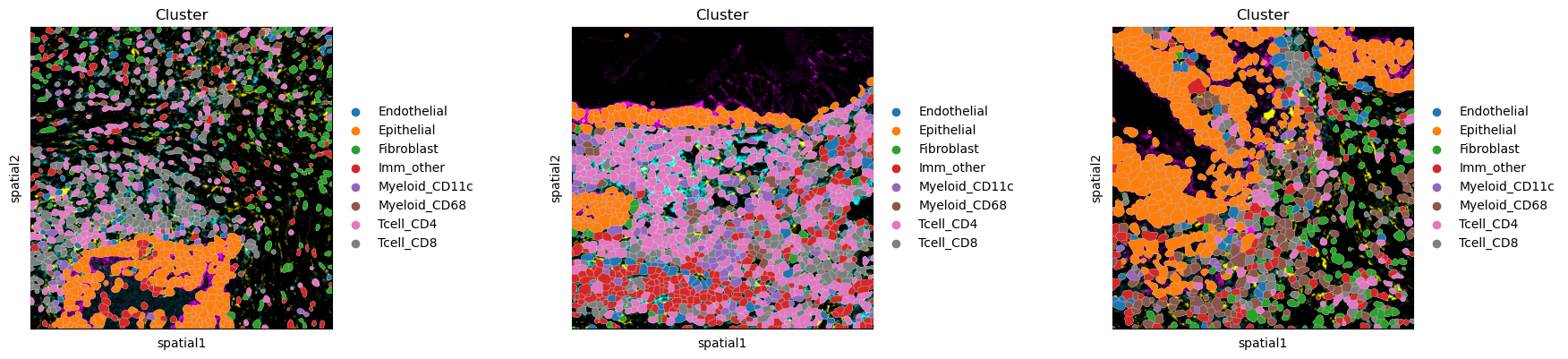
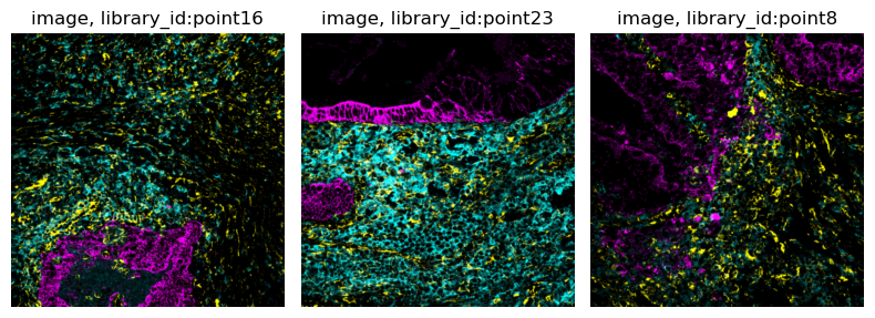
The subset of the data we consider here comprises three biopsies colorectal carcinoma biopsies from different donors, where MIBI-TOF was used to measure single-cell metabolic profiles. As imaging information, we included three raw image channels:

• 145_CD45 - a immune cell marker (cyan).

• 174_CK - a tumor marker (magenta).

• 113_vimentin - a mesenchymal cell marker (yellow).

and a cell segmentation mask provided by the authors of the original paper.

The adata object contains three different libraries, one for each biopsy. The images are contained in adata.uns['spatial'][<library_id>]['images']. Let us visualize the cluster annotations for each library using squidpy.pl.spatial_scatter().

sq.pl.spatial_segment(
    adata, color="Cluster", library_key="library_id", seg_cell_id="cell_id"
)

Let us create an ImageContainer from the images contained in adata. As all three biopsies are already joined in adata, let us also create one ImageContainer for all three biopsies using a z-stack. For more information on how to use ImageContainer with z-stacks, also have a look at Use z-stacks with ImageContainer.

imgs = []
for library_id in adata.uns["spatial"].keys():
    img = sq.im.ImageContainer(
        adata.uns["spatial"][library_id]["images"]["hires"], library_id=library_id
    )
    img.add_img(
        adata.uns["spatial"][library_id]["images"]["segmentation"],
        library_id=library_id,
        layer="segmentation",
    )
    img["segmentation"].attrs["segmentation"] = True
    imgs.append(img)
img = sq.im.ImageContainer.concat(imgs)

WARNING: Channel dimension cannot be aligned with an existing one, using `channels_0`
WARNING: Channel dimension cannot be aligned with an existing one, using `channels_0`
WARNING: Channel dimension cannot be aligned with an existing one, using `channels_0`

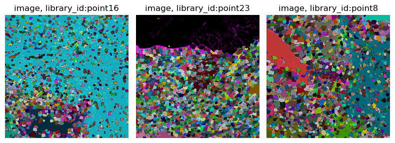
Note that we also added the segmentation as an additional layer to img, and set the segmentation attribute in the ImageContainer. This allows visualization of the segmentation layer as a labels layer in Napari.

img

ImageContainer object with 2 layers:

image: y (1024), x (1024), z (3), channels (3)

segmentation: y (1024), x (1024), z (3), channels_0 (1)

If you have Napari installed, you can have a look at the data using the interactive viewer: Note that you can load the segmentation layer as an overlay over the image.

.. code-block:: python

img.interactive(adata, library_key='library_id')

Let us also statically visualize the data in img, using squidpy.im.ImageCntainer.show():

img.show("image")
img.show("image", segmentation_layer="segmentation")

In the following we show how to use Squidpy to extract cellular mean intensity information using raw images and a provided segmentation mask. In the present case, adata of course already contains the post-processed cellular mean intensity for the raw image channels. The aim of this tutorial, however, is to showcase how the extraction of such features is possible using Squidpy. As Squidpy is backed by dask and supports chunked image processing, also large images can be processed in this way.

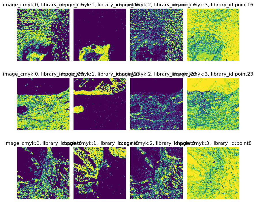
Convert image to CMYK

As already mentioned, the images contain information from three raw channels, 145_CD45, 174_CK, and 113_vimentin. As the channel information is encoded in CMYK space, we first need to convert the RGB images to CMYK.

For this, we can use squidpy.im.ImageContainer.apply().

def rgb2cmyk(arr):
    """Convert arr from RGB to CMYK color space."""
    R = arr[..., 0] / 255
    G = arr[..., 1] / 255
    B = arr[..., 2] / 255
    K = 1 - (np.max(arr, axis=-1) / 255)
    C = (1 - R - K) / (1 - K + np.finfo(float).eps)  # avoid division by 0
    M = (1 - G - K) / (1 - K + np.finfo(float).eps)
    Y = (1 - B - K) / (1 - K + np.finfo(float).eps)
    return np.stack([C, M, Y, K], axis=3)


img.apply(rgb2cmyk, layer="image", new_layer="image_cmyk", copy=False)
img.show("image_cmyk", channelwise=True)

WARNING: Channel dimension cannot be aligned with an existing one, using `channels_1`

Extract per-cell mean intensity

Now that we have disentangled the individual channels, let use use the provided segmentation mask to extract per-cell mean intensities.

By default, the segmentation feature extractor extracts information using all segments (cells) in the current crop. As we would like to only get information of the segment (cell) in the center of the current crop, let us use a custom feature extractor.

Fist, define a custom feature extraction function. This function needs to get the segmentation mask and the original image as input. We will achieve this by passing an additional_layers argument to the custom feature extractor. This special argument will pass the values of every layer in additional_layers to the custom feature extraction function.

def segmentation_image_intensity(arr, image_cmyk):
    """
    Calculate per-channel mean intensity of the center segment.

    arr: the segmentation
    image_cmyk: the raw image values
    """
    import skimage.measure

    # the center of the segmentation mask contains the current label
    # use that to calculate the mask
    s = arr.shape[0]
    mask = (arr == arr[s // 2, s // 2, 0, 0]).astype(int)
    # use skimage.measure.regionprops to get the intensity per channel
    features = []
    for c in range(image_cmyk.shape[-1]):
        feature = skimage.measure.regionprops_table(
            np.squeeze(mask),  # skimage needs 3d or 2d images, so squeeze excess dims
            intensity_image=np.squeeze(image_cmyk[:, :, :, c]),
            properties=["mean_intensity"],
        )["mean_intensity"][0]
        features.append(feature)
    return features

Now, use squidpy.im.calculate_image_features() with the custom feature extractor, specifying the function (func) to use, and the additional layers (additional_layers) to pass to the function. We will use spot_scale = 10 to ensure that we also cover big segments fully by one crop.

sq.im.calculate_image_features(
    adata,
    img,
    library_id="library_id",
    features="custom",
    spot_scale=10,
    layer="segmentation",
    features_kwargs={
        "custom": {
            "func": segmentation_image_intensity,
            "additional_layers": ["image_cmyk"],
        }
    },
)

100%|██████████| 3309/3309 [00:26<00:00, 126.91/s]

The resulting features are stored in adata.obs['img_features'], with channel 0 representing 145_CD45, channel 1 174_CK, and channel 2 113_vimentin.

adata.obsm["img_features"]

	segmentation_image_intensity_0	segmentation_image_intensity_1	segmentation_image_intensity_2	segmentation_image_intensity_3
3034-0	0.000000	0.995041	0.010664	0.492503
3035-0	0.000049	0.884839	0.042991	0.713101
3036-0	0.680350	0.000235	0.222640	0.948284
3037-0	0.813055	0.000000	0.173941	0.790169
3038-0	0.420203	0.015063	0.486171	0.709584
...	...	...	...	...
47342-2	0.000000	0.000000	0.696113	0.855720
47343-2	0.441017	0.000000	0.587986	0.941870
47344-2	0.639157	0.000000	0.344870	0.858989
47345-2	0.196760	0.000000	0.612479	0.855991
47346-2	0.000000	0.000000	0.774775	0.981311

3309 rows × 4 columns

As described in [Hartmann et al., 2020], let us transformed using an inverse hyperbolic sine (arcsinh) co-factor of 0.05, to allow us to compare the computed mean intensities with the values contained in adata.

adata.obsm["img_features_transformed"] = np.arcsinh(adata.obsm["img_features"] / 0.05)

Now, let’s visualize the result:

channels = ["CD45", "CK", "vimentin"]

fig, axes = plt.subplots(1, 3, figsize=(15, 3))
for i, ax in enumerate(axes):
    X = np.array(adata[:, channels[i]].X.todense())[:, 0]
    Y = adata.obsm["img_features_transformed"][f"segmentation_image_intensity_{i}"]
    ax.scatter(X, Y)
    ax.set_xlabel("true value in adata.X")
    ax.set_ylabel("computed mean intensity")
    corr = np.corrcoef(X, Y)[1, 0]
    ax.set_title(f"{channels[i]}, corr: {corr:.2f}")

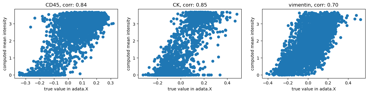
We get high correlations between the original values and our computation using Squidpy. The remaining differences are probably due to more pre-processing applied by the authors of [Hartmann et al., 2020].

In this tutorial we have shown how to pre-process imaging data to extract per-cell counts / mean intensities using Squidpy. Of course it is also possible to apply spatial statistics functions provided by the squidpy.gr module to MIBI-TOF data. For examples of this, please see our other Analysis tutorials, e.g. Analyze seqFISH data.