%matplotlib inline

Analyze Merfish data

This tutorial shows how to apply Squidpy for the analysis of Merfish data.

The data used here was obtained from [Moffitt et al., 2018]. We provide a pre-processed subset of the data, in anndata.AnnData format. For details on how it was pre-processed, please refer to the original paper.

Import packages & data

To run the notebook locally, create a conda environment as conda env create -f environment.yml using this environment.yml <https://github.com/scverse/squidpy_notebooks/blob/main/environment.yml>_.

import scanpy as sc
import squidpy as sq

sc.logging.print_header()
print(f"squidpy=={sq.__version__}")

# load the pre-processed dataset
adata = sq.datasets.merfish()
adata

scanpy==1.9.2 anndata==0.8.0 umap==0.5.3 numpy==1.21.0 scipy==1.9.3 pandas==1.5.1 scikit-learn==1.1.3 statsmodels==0.13.2 python-igraph==0.10.2 pynndescent==0.5.7
squidpy==1.2.2

100%|██████████| 49.2M/49.2M [00:07<00:00, 7.05MB/s]

AnnData object with n_obs × n_vars = 73655 × 161
    obs: 'Cell_ID', 'Animal_ID', 'Animal_sex', 'Behavior', 'Bregma', 'Centroid_X', 'Centroid_Y', 'Cell_class', 'Neuron_cluster_ID', 'batch'
    uns: 'Cell_class_colors'
    obsm: 'spatial', 'spatial3d'

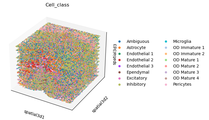
This datasets consists of consecutive slices from the mouse hypothalamic preoptic region. It represents an interesting example of how to work with 3D spatial data in Squidpy. Let’s start with visualization: we can either visualize the 3D stack of slides using scanpy.pl.embedding():

sc.pl.embedding(adata, basis="spatial3d", projection="3d", color="Cell_class")

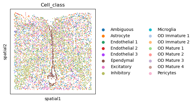
Or visualize a single slide with squidpy.pl.spatial_scatter(). Here the slide identifier is stored in adata.obs["Bregma"], see original paper for definition.

sq.pl.spatial_scatter(
    adata[adata.obs.Bregma == -9], shape=None, color="Cell_class", size=1
)

WARNING: Please specify a valid `library_id` or set it permanently in `adata.uns['spatial']`

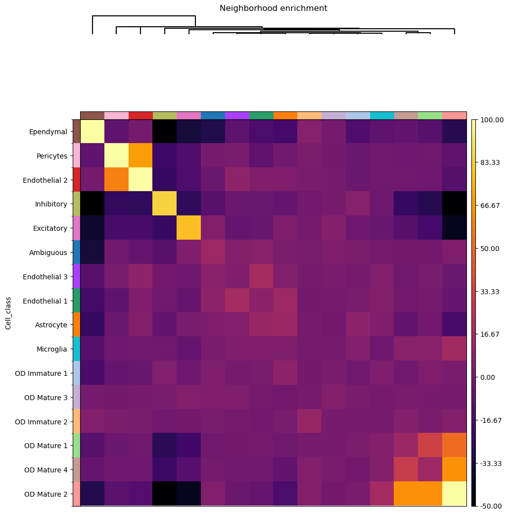
Neighborhood enrichment analysis in 3D

It is important to consider whether the analysis should be performed on the 3D spatial coordinates or the 2D coordinates for a single slice. Functions that make use of the spatial graph can already support 3D coordinates, but it is important to consider that the z-stack coordinate is in the same unit metrics as the x, y coordinates. Let’s start with the neighborhood enrichment score. You can read more on the function in the docs at Building spatial neighbors graph. First, we need to compute a neighbor graph with squidpy.gr.spatial_neighbors(). If we want to compute the neighbor graph on the 3D coordinate space, we need to specify spatial_key = "spatial3d". Then we can use squidpy.gr.nhood_enrichment() to compute the score, and visualize it with squidpy.gr.nhood_enrichment().

sq.gr.spatial_neighbors(adata, coord_type="generic", spatial_key="spatial3d")
sq.gr.nhood_enrichment(adata, cluster_key="Cell_class")
sq.pl.nhood_enrichment(
    adata, cluster_key="Cell_class", method="single", cmap="inferno", vmin=-50, vmax=100
)

100%|██████████| 1000/1000 [00:11<00:00, 88.86/s]

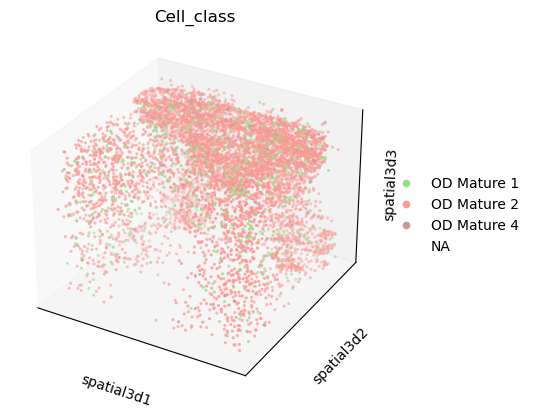
We can visualize some of the co-enriched clusters with scanpy.pl.embedding(). We will set na_colors=(1,1,1,0) to make transparent the other observations, in order to better visualize the clusters of interests across z-stacks.

sc.pl.embedding(
    adata,
    basis="spatial3d",
    groups=["OD Mature 1", "OD Mature 2", "OD Mature 4"],
    na_color=(1, 1, 1, 0),
    projection="3d",
    color="Cell_class",
)

We can also visualize gene expression in 3D coordinates. Let’s perform differential expression testing with scanpy.tl.rank_genes_groups() and visualize the results

sc.tl.rank_genes_groups(adata, groupby="Cell_class")
sc.pl.rank_genes_groups(adata, groupby="Cell_class")

WARNING: Default of the method has been changed to 't-test' from 't-test_overestim_var'

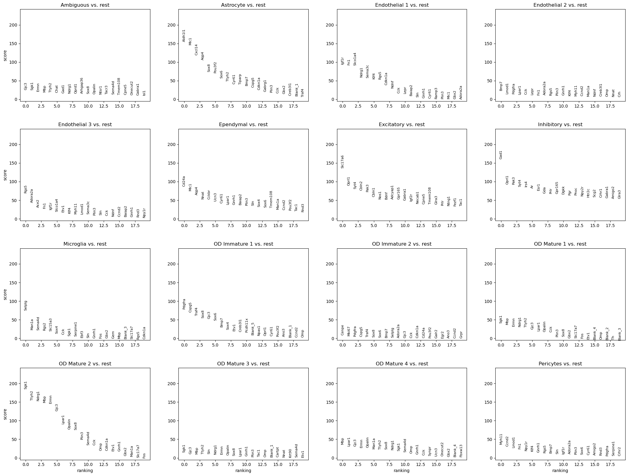
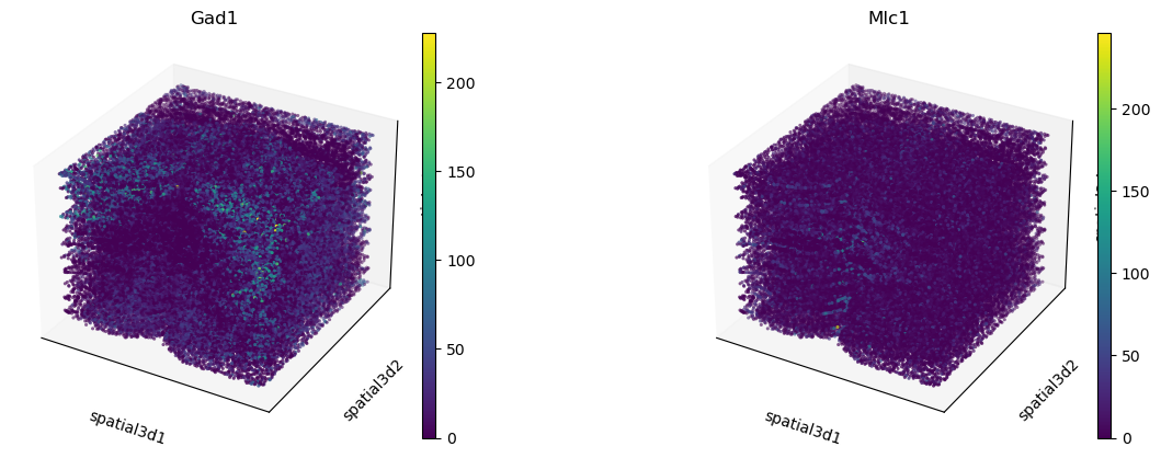
and the expression in 3D.

sc.pl.embedding(adata, basis="spatial3d", projection="3d", color=["Gad1", "Mlc1"])

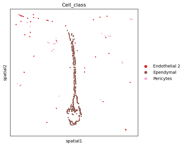
If the same analysis should be performed on a single slice, then it is advisable to copy the sample of interest in a new anndata.AnnData and use it as a standard 2D spatial data object.

adata_slice = adata[adata.obs.Bregma == -9].copy()
sq.gr.spatial_neighbors(adata_slice, coord_type="generic")
sq.gr.nhood_enrichment(adata, cluster_key="Cell_class")
sq.pl.spatial_scatter(
    adata_slice,
    color="Cell_class",
    shape=None,
    groups=[
        "Ependymal",
        "Pericytes",
        "Endothelial 2",
    ],
    size=10,
)

100%|██████████| 1000/1000 [00:11<00:00, 87.51/s]

WARNING: Please specify a valid `library_id` or set it permanently in `adata.uns['spatial']`

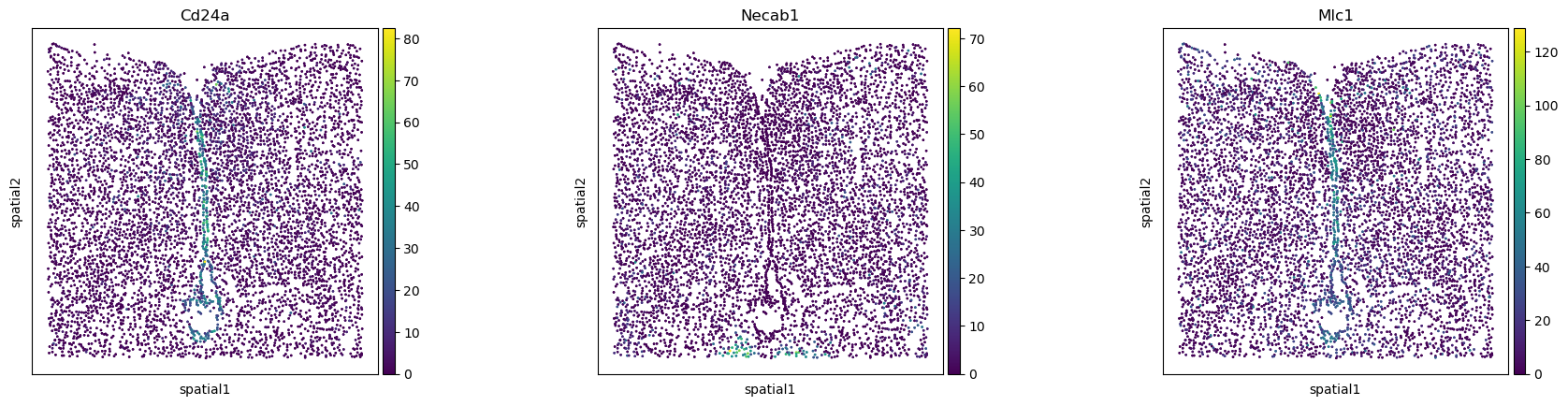
Spatially variable genes with spatial autocorrelation statistics

With Squidpy we can investigate spatial variability of gene expression. This is an example of a function that only supports 2D data. squidpy.gr.spatial_autocorr() conveniently wraps two spatial autocorrelation statistics: Moran’s I and Geary’s C. They provide a score on the degree of spatial variability of gene expression. The statistic as well as the p-value are computed for each gene, and FDR correction is performed. For the purpose of this tutorial, let’s compute the Moran’s I score. The results are stored in adata.uns['moranI'] and we can visualize selected genes with squidpy.pl.spatial_scatter().

sq.gr.spatial_autocorr(adata_slice, mode="moran")
adata_slice.uns["moranI"].head()
sq.pl.spatial_scatter(
    adata_slice, shape=None, color=["Cd24a", "Necab1", "Mlc1"], size=3
)

WARNING: Please specify a valid `library_id` or set it permanently in `adata.uns['spatial']`