%matplotlib inline
Building spatial neighbors graph
This example shows how to compute a spatial neighbors graph.
Spatial graph is a graph of spatial neighbors with observations as nodes and neighbor-hood relations between observations as edges. We use spatial coordinates of spots/cells to identify neighbors among them. Different approach of defining a neighborhood relation among observations are used for different types of spatial datasets.
import numpy as np

import squidpy as sq
First, we show how to compute the spatial neighbors graph for a Visium dataset.
adata = sq.datasets.visium_fluo_adata()
adata
AnnData object with n_obs × n_vars = 2800 × 16562
    obs: 'in_tissue', 'array_row', 'array_col', 'n_genes_by_counts', 'log1p_n_genes_by_counts', 'total_counts', 'log1p_total_counts', 'pct_counts_in_top_50_genes', 'pct_counts_in_top_100_genes', 'pct_counts_in_top_200_genes', 'pct_counts_in_top_500_genes', 'total_counts_MT', 'log1p_total_counts_MT', 'pct_counts_MT', 'n_counts', 'leiden', 'cluster'
    var: 'gene_ids', 'feature_types', 'genome', 'MT', 'n_cells_by_counts', 'mean_counts', 'log1p_mean_counts', 'pct_dropout_by_counts', 'total_counts', 'log1p_total_counts', 'n_cells', 'highly_variable', 'highly_variable_rank', 'means', 'variances', 'variances_norm'
    uns: 'cluster_colors', 'hvg', 'leiden', 'leiden_colors', 'neighbors', 'pca', 'spatial', 'umap'
    obsm: 'X_pca', 'X_umap', 'spatial'
    varm: 'PCs'
    obsp: 'connectivities', 'distances'
We use squidpy.gr.spatial_neighbors() for this. The function expects
coord_type = 'visium' by default. We set this parameter here
explicitly for clarity. n_rings should be used only for Visium
datasets. It specifies for each spot how many hexagonal rings of spots
around will be considered neighbors.
sq.gr.spatial_neighbors(adata, n_rings=2, coord_type="grid", n_neighs=6)
The function builds a spatial graph and saves its adjacency matrix to
adata.obsp['spatial_connectivities'] and weighted adjacency matrix to
adata.obsp['spatial_distances'] by default. Note that it can also
build a a graph from a square grid, just set n_neighs = 4.
adata.obsp["spatial_connectivities"]
<2800x2800 sparse matrix of type '<class 'numpy.float64'>'
	with 48240 stored elements in Compressed Sparse Row format>
The weights of the weighted adjacency matrix are ordinal numbers of
hexagonal rings in the case of coord_type = 'visium'.
adata.obsp["spatial_distances"]
<2800x2800 sparse matrix of type '<class 'numpy.float64'>'
	with 48240 stored elements in Compressed Sparse Row format>
We can visualize the neighbors of a point to better visualize what [n_rings]{.title-ref} mean:
_, idx = adata.obsp["spatial_connectivities"][420, :].nonzero()
idx = np.append(idx, 420)
sq.pl.spatial_scatter(
    adata[idx, :],
    connectivity_key="spatial_connectivities",
    img=False,
    na_color="lightgrey",
)

Next, we show how to compute the spatial neighbors graph for a non-grid dataset.
adata = sq.datasets.imc()
adata
AnnData object with n_obs × n_vars = 4668 × 34
    obs: 'cell type'
    uns: 'cell type_colors'
    obsm: 'spatial'
We use the same function for this with coord_type = 'generic'.
n_neighs and radius can be used for non-Visium datasets. n_neighs
specifies a fixed number of the closest spots for each spot as
neighbors. Alternatively, delaunay = True can be used, for a Delaunay
triangulation graph.
sq.gr.spatial_neighbors(adata, n_neighs=10, coord_type="generic")
_, idx = adata.obsp["spatial_connectivities"][420, :].nonzero()
idx = np.append(idx, 420)
sq.pl.spatial_scatter(
    adata[idx, :],
    shape=None,
    color="cell type",
    connectivity_key="spatial_connectivities",
    size=100,
)
WARNING: Please specify a valid `library_id` or set it permanently in {attr}`adata.uns['spatial']`
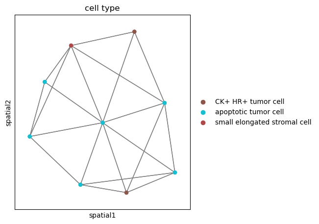
We use the same function for this with coord_type = 'generic' and
delaunay = True. You can appreciate that the neighbor graph is
slightly different than before.
sq.gr.spatial_neighbors(adata, delaunay=True, coord_type="generic")
_, idx = adata.obsp["spatial_connectivities"][420, :].nonzero()
idx = np.append(idx, 420)
sq.pl.spatial_scatter(
    adata[idx, :],
    shape=None,
    color="cell type",
    connectivity_key="spatial_connectivities",
    size=100,
)
WARNING: Please specify a valid `library_id` or set it permanently in {attr}`adata.uns['spatial']`

In order to get all spots within a specified radius (in units of the
spatial coordinates) from each spot as neighbors, the parameter radius
should be used.
sq.gr.spatial_neighbors(adata, radius=0.3, coord_type="generic")

adata.obsp["spatial_connectivities"]
adata.obsp["spatial_distances"]
<4668x4668 sparse matrix of type '<class 'numpy.float64'>'
	with 0 stored elements in Compressed Sparse Row format>