%matplotlib inline

Compute Ripley’s statistics

This example shows how to compute the Ripley’s L function.

The Ripley’s L function is a descriptive statistics generally used to determine whether points have a random, dispersed or clustered distribution pattern at certain scale. The Ripley’s L is a variance-normalized version of the Ripley’s K statistic.

See also

See {doc}`compute_co_occurrence` for
another score to describe spatial patterns with {func}`squidpy.gr.co_occurrence`.

import squidpy as sq

adata = sq.datasets.slideseqv2()
adata

AnnData object with n_obs × n_vars = 41786 × 4000
    obs: 'barcode', 'x', 'y', 'n_genes_by_counts', 'log1p_n_genes_by_counts', 'total_counts', 'log1p_total_counts', 'pct_counts_in_top_50_genes', 'pct_counts_in_top_100_genes', 'pct_counts_in_top_200_genes', 'pct_counts_in_top_500_genes', 'total_counts_MT', 'log1p_total_counts_MT', 'pct_counts_MT', 'n_counts', 'leiden', 'cluster'
    var: 'MT', 'n_cells_by_counts', 'mean_counts', 'log1p_mean_counts', 'pct_dropout_by_counts', 'total_counts', 'log1p_total_counts', 'n_cells', 'highly_variable', 'highly_variable_rank', 'means', 'variances', 'variances_norm'
    uns: 'cluster_colors', 'hvg', 'leiden', 'leiden_colors', 'neighbors', 'pca', 'spatial_neighbors', 'umap'
    obsm: 'X_pca', 'X_umap', 'deconvolution_results', 'spatial'
    varm: 'PCs'
    obsp: 'connectivities', 'distances', 'spatial_connectivities', 'spatial_distances'

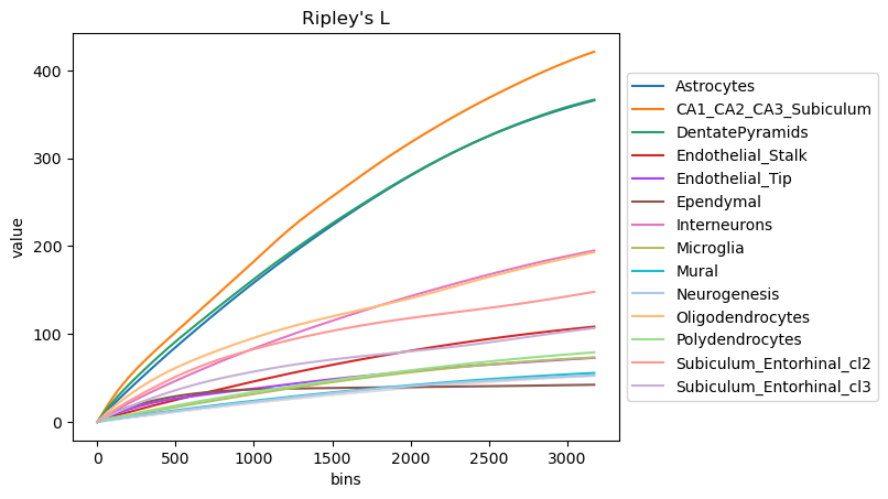
We can compute the Ripley’s L function with squidpy.gr.ripley(). Results can be visualized with squidpy.pl.ripley().

mode = "L"
sq.gr.ripley(adata, cluster_key="cluster", mode=mode)
sq.pl.ripley(adata, cluster_key="cluster", mode=mode)

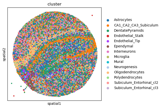
We can further visualize tissue organization in spatial coordinates with squidpy.pl.spatial_scatter().

sq.pl.spatial_scatter(adata, color="cluster", size=20, shape=None)

WARNING: Please specify a valid `library_id` or set it permanently in {attr}`adata.uns['spatial']`

There are also 2 other Ripley’s statistics available (that are closely related): mode = 'F' and mode = 'G'.