%matplotlib inline

Crop images with ImageContainer

This example shows how crop images from squidpy.im.ImageContainer.

Specifically, it shows how to use:

• squidpy.im.ImageContainer.crop_corner()

• squidpy.im.ImageContainer.crop_center()

import matplotlib.pyplot as plt

import squidpy as sq

Let’s load the fluorescence Visium image.

img = sq.datasets.visium_fluo_image_crop()

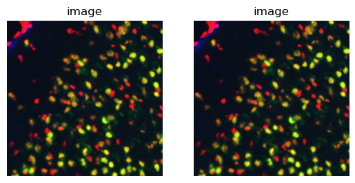
Extracting single crops: Crops need to be sized and located. We distinguish crops located based on a corner coordinate of the crop and crops located based on the center coordinate of the crop. You can specify the crop coordinates in pixels (as int) or in percentage of total image size (as float). In addition, you can specify a scaling factor for the crop.

crop_corner = img.crop_corner(1000, 1000, size=800)

crop_center = img.crop_center(1400, 1400, radius=400)

fig, axes = plt.subplots(1, 2)
crop_corner.show(ax=axes[0])
crop_center.show(ax=axes[1])

The result of the cropping functions is another ImageContainer.

crop_corner

ImageContainer object with 1 layer:

image: y (800), x (800), z (1), channels (3)

You can subset the associated adata to the cropped image using squidpy.im.ImageContainer.subset():

adata = sq.datasets.visium_fluo_adata_crop()
adata

AnnData object with n_obs × n_vars = 704 × 16562
    obs: 'in_tissue', 'array_row', 'array_col', 'n_genes_by_counts', 'log1p_n_genes_by_counts', 'total_counts', 'log1p_total_counts', 'pct_counts_in_top_50_genes', 'pct_counts_in_top_100_genes', 'pct_counts_in_top_200_genes', 'pct_counts_in_top_500_genes', 'total_counts_MT', 'log1p_total_counts_MT', 'pct_counts_MT', 'n_counts', 'leiden', 'cluster'
    var: 'gene_ids', 'feature_types', 'genome', 'MT', 'n_cells_by_counts', 'mean_counts', 'log1p_mean_counts', 'pct_dropout_by_counts', 'total_counts', 'log1p_total_counts', 'n_cells', 'highly_variable', 'highly_variable_rank', 'means', 'variances', 'variances_norm'
    uns: 'cluster_colors', 'hvg', 'leiden', 'leiden_colors', 'neighbors', 'pca', 'spatial', 'umap'
    obsm: 'X_pca', 'X_umap', 'spatial'
    varm: 'PCs'
    obsp: 'connectivities', 'distances'

Note the number of observations in adata before and after subsetting.

adata_crop = crop_corner.subset(adata)
adata_crop

View of AnnData object with n_obs × n_vars = 7 × 16562
    obs: 'in_tissue', 'array_row', 'array_col', 'n_genes_by_counts', 'log1p_n_genes_by_counts', 'total_counts', 'log1p_total_counts', 'pct_counts_in_top_50_genes', 'pct_counts_in_top_100_genes', 'pct_counts_in_top_200_genes', 'pct_counts_in_top_500_genes', 'total_counts_MT', 'log1p_total_counts_MT', 'pct_counts_MT', 'n_counts', 'leiden', 'cluster'
    var: 'gene_ids', 'feature_types', 'genome', 'MT', 'n_cells_by_counts', 'mean_counts', 'log1p_mean_counts', 'pct_dropout_by_counts', 'total_counts', 'log1p_total_counts', 'n_cells', 'highly_variable', 'highly_variable_rank', 'means', 'variances', 'variances_norm'
    uns: 'cluster_colors', 'hvg', 'leiden', 'leiden_colors', 'neighbors', 'pca', 'spatial', 'umap'
    obsm: 'X_pca', 'X_umap', 'spatial'
    varm: 'PCs'
    obsp: 'connectivities', 'distances'

Visualize the result in Napari:

crop_corner.interactive(adata_crop)