%matplotlib inline

Process a high-resolution image

This example shows how to use squidpy.im.process with tiling.

The function can be applied to any method (e.g., smoothing, conversion to grayscale) or layer of a high-resolution image layer of squidpy.im.ImageContainer.

By default, squidpy.im.process processes the entire input image at once. In the case of high-resolution tissue slides however, the images might be too big to fit in memory and cannot be processed at once. In that case you can use the argument chunks to tile the image in crops of shape chunks, process each crop, and re-assemble the resulting image. Note that you can also use squidpy.im.segment in this manner.

Note that depending on the processing function used, there might be border effects occurring at the edges of the crops. Since Squidpy is backed by dask, and internally chunking is done using dask.array.map_overlap, dealing with these border effects is easy. Just specify the depth and boundary arguments in the apply_kwargs upon the call to squidpy.im.process. For more information, please refer to the documentation of dask.array.map_overlap.

For the build in processing functions, [gray]{.title-ref} and [smooth]{.title-ref}, the border effects are already automatically taken care of, so it is not necessary to specify depth and boundary. For squidpy.im.segment, the default depth is 30, which already takes care of most severe border effects.

See also

• examples_image_compute_smooth.

• examples_image_compute_gray.

• examples_image_compute_segment_fluo.

import numpy as np
from scipy.ndimage import gaussian_filter

import matplotlib.pyplot as plt

import squidpy as sq

Built-in processing functions

# load the H&E stained tissue image
img = sq.datasets.visium_hne_image()

We will process the image by tiling it in crops of shape chunks = (1000, 1000).

sq.im.process(img, layer="image", method="gray", chunks=1000)

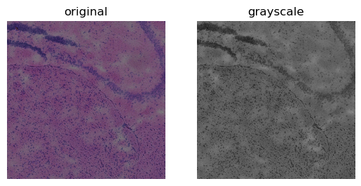
Now we can look at the result on a cropped part of the image.

crop = img.crop_corner(4000, 4000, size=2000)

fig, axes = plt.subplots(1, 2)
crop.show("image", ax=axes[0])
_ = axes[0].set_title("original")
crop.show("image_gray", cmap="gray", ax=axes[1])
_ = axes[1].set_title("grayscale")

Custom processing functions

Here, we use a custom processing function (here scipy.ndimage.gaussian_filter) with chunking to showcase the depth and boundary arguments.

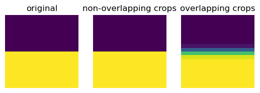
Lets use a simple image and choose the chunk size in such a way to clearly see the differences between using overlapping crops and non-overlapping crops.

arr = np.zeros((20, 20))
arr[10:] = 1
img = sq.im.ImageContainer(arr, layer="image")

# smooth the image using `depth` 0 and 1
sq.im.process(
    img,
    layer="image",
    method=gaussian_filter,
    layer_added="smooth_depth0",
    chunks=10,
    sigma=1,
    apply_kwargs={"depth": 0},
)
sq.im.process(
    img,
    layer="image",
    method=gaussian_filter,
    layer_added="smooth_depth1",
    chunks=10,
    sigma=1,
    apply_kwargs={"depth": 1, "boundary": "reflect"},
)

Plot the difference in results. Using overlapping blocks with depth = 1 removes the artifacts at the borders between chunks.

fig, axes = plt.subplots(1, 3)
img.show("image", ax=axes[0])
_ = axes[0].set_title("original")
img.show("smooth_depth0", ax=axes[1])
_ = axes[1].set_title("non-overlapping crops")
img.show("smooth_depth1", ax=axes[2])
_ = axes[2].set_title("overlapping crops")