%matplotlib inline

Use z-stacks with ImageContainer

In this example we showcase how to use z-stacks with squidpy.im.ImageContainer

It is possible to acquire several consecutive image slices from the same tissue. Squidpy’s ImageContainer supports storing, processing, and visualization of these z-stacks.

Here, we use the Visium 10x mouse brain sagittal slices as an example of a z-stack image with two Z dimensions. We will use the “hires” images contained in the anndata.AnnData object, but you could also use the original resolution tiff images in the ImageContainer.

Import libraries and load individual image sections

import anndata as ad
import scanpy as sc
import squidpy as sq

library_ids = [
    "V1_Mouse_Brain_Sagittal_Posterior",
    "V1_Mouse_Brain_Sagittal_Posterior_Section_2",
]

adatas, imgs = [], []
use_hires_tiff = False
for library_id in library_ids:
    adatas.append(sc.datasets.visium_sge(library_id, include_hires_tiff=use_hires_tiff))
    adatas[-1].var_names_make_unique()
    if use_hires_tiff:
        imgs.append(
            sq.im.ImageContainer(
                adatas[-1].uns["spatial"][library_id]["metadata"]["source_image_path"]
            )
        )
    else:
        # as we are using a scaled image, we need to specify a scalefactor
        # to allow correct mapping to adata.obsm['spatial']
        imgs.append(
            sq.im.ImageContainer(
                adatas[-1].uns["spatial"][library_id]["images"]["hires"],
                scale=adatas[-1].uns["spatial"][library_id]["scalefactors"][
                    "tissue_hires_scalef"
                ],
            )
        )

100%|██████████| 9.26M/9.26M [00:01<00:00, 4.96MB/s]
100%|██████████| 20.1M/20.1M [00:05<00:00, 3.57MB/s]
100%|██████████| 9.26M/9.26M [00:01<00:00, 5.00MB/s]
100%|██████████| 19.0M/19.0M [00:04<00:00, 4.66MB/s]

Concatenate per-section data to a z-stack

To allow mapping from observations in adata to the correct Z dimension in img, we will store a library_id column in adata.obs and associate each library_id to a Z dimension in the ImageContainer.

For this, we will use anndata.concat() with uns_merge = only (to ensure that uns entries are correctly concatenated), label = 'library_id' and keys = library_ids (to create the necessary column in adata.obs.

To concatenate the individual squidpy.im.ImageContainer, we will use squidpy.im.ImageContainer.concat(), specifying library_ids = library_ids for associating each image with the correct observations in adata.

adata = ad.concat(
    adatas, uns_merge="only", label="library_id", keys=library_ids, index_unique="-"
)
img = sq.im.ImageContainer.concat(imgs, library_ids=library_ids)

adata now contains a library_id column in adata.obs, which maps observations to a unique library_id.

print(adata)
adata.obs

AnnData object with n_obs × n_vars = 6644 × 32285
    obs: 'in_tissue', 'array_row', 'array_col', 'library_id'
    uns: 'spatial'
    obsm: 'spatial'

	in_tissue	array_row	array_col	library_id
AAACAAGTATCTCCCA-1-V1_Mouse_Brain_Sagittal_Posterior	1	50	102	V1_Mouse_Brain_Sagittal_Posterior
AAACACCAATAACTGC-1-V1_Mouse_Brain_Sagittal_Posterior	1	59	19	V1_Mouse_Brain_Sagittal_Posterior
AAACAGAGCGACTCCT-1-V1_Mouse_Brain_Sagittal_Posterior	1	14	94	V1_Mouse_Brain_Sagittal_Posterior
AAACAGCTTTCAGAAG-1-V1_Mouse_Brain_Sagittal_Posterior	1	43	9	V1_Mouse_Brain_Sagittal_Posterior
AAACAGGGTCTATATT-1-V1_Mouse_Brain_Sagittal_Posterior	1	47	13	V1_Mouse_Brain_Sagittal_Posterior
...	...	...	...	...
TTGTTGTGTGTCAAGA-1-V1_Mouse_Brain_Sagittal_Posterior_Section_2	1	31	77	V1_Mouse_Brain_Sagittal_Posterior_Section_2
TTGTTTCACATCCAGG-1-V1_Mouse_Brain_Sagittal_Posterior_Section_2	1	58	42	V1_Mouse_Brain_Sagittal_Posterior_Section_2
TTGTTTCATTAGTCTA-1-V1_Mouse_Brain_Sagittal_Posterior_Section_2	1	60	30	V1_Mouse_Brain_Sagittal_Posterior_Section_2
TTGTTTCCATACAACT-1-V1_Mouse_Brain_Sagittal_Posterior_Section_2	1	45	27	V1_Mouse_Brain_Sagittal_Posterior_Section_2
TTGTTTGTATTACACG-1-V1_Mouse_Brain_Sagittal_Posterior_Section_2	1	73	41	V1_Mouse_Brain_Sagittal_Posterior_Section_2

6644 rows × 4 columns

img contains the 2D images concatenated along the Z dimension in one image layer. The Z dimensions are named the same as the library_id’s in adata to allow a mapping from adata to img.

print(img["image"].z)
img

<xarray.DataArray 'z' (z: 2)>
array(['V1_Mouse_Brain_Sagittal_Posterior',
       'V1_Mouse_Brain_Sagittal_Posterior_Section_2'], dtype='<U43')
Coordinates:
  * z        (z) <U43 'V1_Mouse_Brain_Sagittal_Posterior' 'V1_Mouse_Brain_Sag...

ImageContainer object with 1 layer:

image: y (1998), x (2000), z (2), channels (3)

It is also possible to initialize the ImageContainer with images that already contain the Z dimension. In this case you need to specify the library_id argument in the constructor. In addition, you might want to set dims to the correct ordering of dimensions manually for more control.

arr = img["image"].values
print(arr.shape)
img2 = sq.im.ImageContainer(
    arr, library_id=library_ids, dims=("y", "x", "z", "channels")
)
img2

(1998, 2000, 2, 3)

ImageContainer object with 1 layer:

image: y (1998), x (2000), z (2), channels (3)

Generally, an ImageContainer with more than one Z dimension can be used in the same way as an ImageContainer with only one Z dimension. In addition, we can specify library_id to cropping, pre-processing, and segmentation functions if we’d like to only process a specific library_id.

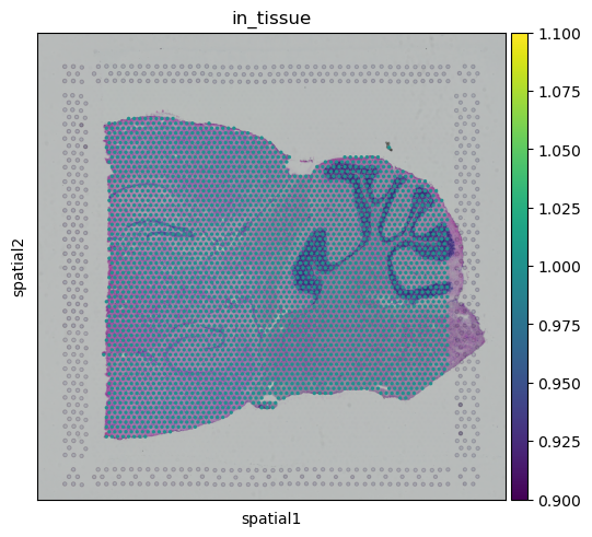
Visualization

For using squidpy.pl.spatial_scatter(), subset the adata to the desired library_id.

library_id = library_ids[0]
sq.pl.spatial_scatter(
    adata[adata.obs["library_id"] == library_id],
    library_id=library_id,
    color="in_tissue",
)

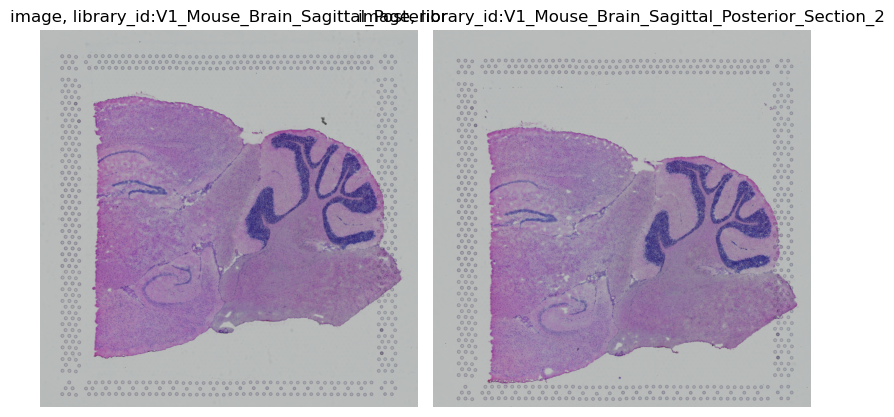
squidpy.im.ImageContainer.show() works with z-stacks out of the box, by plotting them as separate images. Additionally, you can specify a library_id if you only want to plot one Z dimension.

img.show()

Interactive visualization of z-stacks is also possible. The Napari viewer will have a slider at the bottom, allowing you to choose the Z dimension to display. The adata observations are automatically updated to the current Z dimension.

When calling img.interactive just specify library_key as the column name in adata.obs which maps from observations to library_ids

.. code-block:: python

img.interactive(adata, library_key=’library_id’)

Cropping

By default, the cropping functions will crop all Z dimensions.

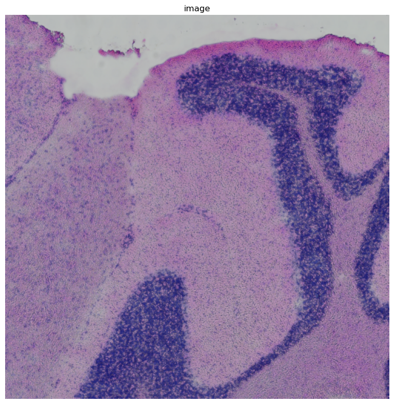
crop = img.crop_corner(500, 1000, size=500)
crop.show()

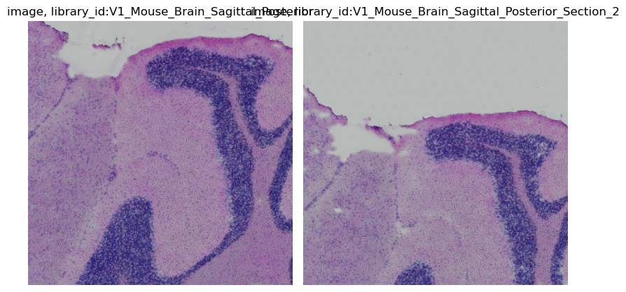
You can also specify library_id, as either a single or multiple Z dimensions to crop.

img.crop_corner(500, 1000, size=500, library_id=library_ids[0]).show()

Processing and segmenting

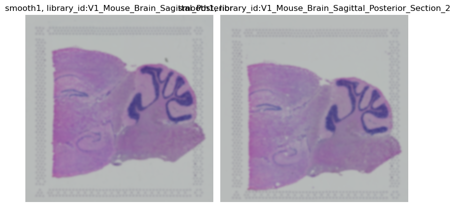
Let us smooth the image. When not specifying a library_id, squidpy.im.process() treats the image as a 3D volume. As we would like to smooth only in x and y dimensions, and not in z, we need so specify a per-dimension sigma. The internal dimensions of the image are y, x, z, channels, as you can check with crop['image'].dims. Therefore, to only smooth in x and y, we need to specify sigma = [10, 10, 0, 0].

sq.im.process(
    img, layer="image", method="smooth", sigma=[10, 10, 0, 0], layer_added="smooth1"
)
img.show("smooth1")

Now, let us just smooth one library_id. Specifying library_id means that the processing function will process each Z dimension separately. This means that now the dimensions of the processed image are y, x, channels (with z removed), meaning that we have to update sigma accordingly. If the number of channels does not change due to the processing, squidpy.im.process() implies the identity function for non-processed Z dimensions.

sq.im.process(
    img,
    layer="image",
    method="smooth",
    sigma=10,
    layer_added="smooth2",
    library_id=library_ids[0],
)
img.show("smooth2")

None, only the first library_id is smoothed. For the second, the original image was used.

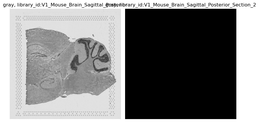
If the processing function changes the number of dimensions, non-processed Z dimensions will contain 0. Let’s see this behavior with using method = 'gray', which moves from 3 channels (RGB) to one channel (gray).

sq.im.process(
    img, layer="image", method="gray", layer_added="gray", library_id=library_ids[0]
)
img.show("gray", cmap="gray")

WARNING: Function changed the number of channels, cannot use identity for library ids `['V1_Mouse_Brain_Sagittal_Posterior_Section_2']`. Replacing with 0

squidpy.im.segment() works in the same way, just specify library_id if you only wish to segment specific Z dimensions.

Feature calculation

Calculating features from z-stack images is straight forward as well. With more than one Z dimension, we just need to specify the column name in adata.obs which contains the mapping from observations to library_ids to allow the function to extract the features from the correct Z dimension. As of now, features can only be extracted on 2D, meaning from the Z dimension that the current spot is located on.

The following call extracts features for each observation in adata, automatically choosing the correct Z dimension in img.

adata_crop = crop.subset(adata)  # subset adata to the image crop
sq.im.calculate_image_features(
    adata_crop,
    crop,
    library_id="library_id",
    layer="image",
    features="summary",
    n_jobs=4,
)
adata_crop.obsm["img_features"]

100%|██████████| 774/774 [00:14<00:00, 54.34/s] 

	summary_ch-0_quantile-0.9	summary_ch-0_quantile-0.5	summary_ch-0_quantile-0.1	summary_ch-0_mean	summary_ch-0_std	summary_ch-1_quantile-0.9	summary_ch-1_quantile-0.5	summary_ch-1_quantile-0.1	summary_ch-1_mean	summary_ch-1_std	summary_ch-2_quantile-0.9	summary_ch-2_quantile-0.5	summary_ch-2_quantile-0.1	summary_ch-2_mean	summary_ch-2_std
AAACAGAGCGACTCCT-1-V1_Mouse_Brain_Sagittal_Posterior	0.721569	0.670588	0.542745	0.647495	0.074835	0.725490	0.611765	0.247059	0.517943	0.209248	0.729412	0.674510	0.549020	0.652933	0.074534
AAACGAGACGGTTGAT-1-V1_Mouse_Brain_Sagittal_Posterior	0.450980	0.309804	0.200000	0.317769	0.095004	0.360784	0.270588	0.184314	0.269996	0.069024	0.576471	0.509804	0.462745	0.515190	0.045777
AAATTACCTATCGATG-1-V1_Mouse_Brain_Sagittal_Posterior	0.680784	0.611765	0.487843	0.599930	0.075161	0.517647	0.462745	0.379608	0.455529	0.055273	0.692549	0.650980	0.596078	0.647303	0.041485
AACAGGAAATCGAATA-1-V1_Mouse_Brain_Sagittal_Posterior	0.658824	0.603922	0.511373	0.594231	0.057229	0.521569	0.466667	0.393725	0.462379	0.048675	0.678431	0.643137	0.584314	0.635939	0.035439
AACATATCAACTGGTG-1-V1_Mouse_Brain_Sagittal_Posterior	0.586667	0.360784	0.211765	0.385795	0.140289	0.447059	0.301961	0.185882	0.308392	0.098326	0.645490	0.533333	0.444706	0.540601	0.071795
...	...	...	...	...	...	...	...	...	...	...	...	...	...	...	...
TTGGGACACTGCCCGC-1-V1_Mouse_Brain_Sagittal_Posterior_Section_2	0.635294	0.580392	0.480000	0.564357	0.063804	0.522353	0.466667	0.397647	0.464401	0.049290	0.674510	0.631373	0.580392	0.627468	0.038752
TTGGGCGGCGGTTGCC-1-V1_Mouse_Brain_Sagittal_Posterior_Section_2	0.643137	0.592157	0.502745	0.582867	0.055017	0.556863	0.505882	0.435294	0.500200	0.047835	0.666667	0.631373	0.581961	0.626580	0.033794
TTGTAAGGCCAGTTGG-1-V1_Mouse_Brain_Sagittal_Posterior_Section_2	0.670588	0.627451	0.537255	0.615948	0.055211	0.602353	0.556863	0.483922	0.548758	0.047661	0.694118	0.662745	0.596078	0.652636	0.036439
TTGTTCAGTGTGCTAC-1-V1_Mouse_Brain_Sagittal_Posterior_Section_2	0.647059	0.584314	0.476078	0.571329	0.064511	0.545098	0.494118	0.419608	0.489499	0.048448	0.674510	0.639216	0.592157	0.636148	0.032888
TTGTTGTGTGTCAAGA-1-V1_Mouse_Brain_Sagittal_Posterior_Section_2	0.662745	0.623529	0.510588	0.607930	0.060086	0.623529	0.568627	0.480000	0.560070	0.054016	0.682353	0.654902	0.607843	0.648872	0.030845

774 rows × 15 columns

The calculated features can now be used in downstream Scanpy analyses, by e.g. using all Z dimensions to cluster spots based on image features and gene features.

Here, we cluster genes and calculated features using a standard Scanpy workflow.

sc.pp.normalize_total(adata_crop, inplace=True)
sc.pp.log1p(adata_crop)
sc.pp.pca(adata_crop)
sc.pp.neighbors(adata_crop)
sc.tl.leiden(adata_crop)

sc.pp.neighbors(adata_crop, use_rep="img_features", key_added="neigh_features")
sc.tl.leiden(adata_crop, neighbors_key="neigh_features", key_added="leiden_features")

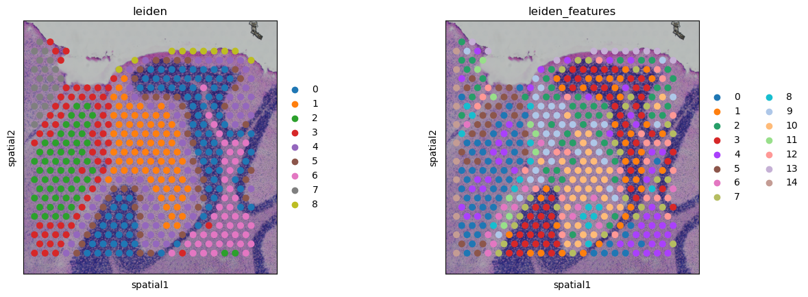
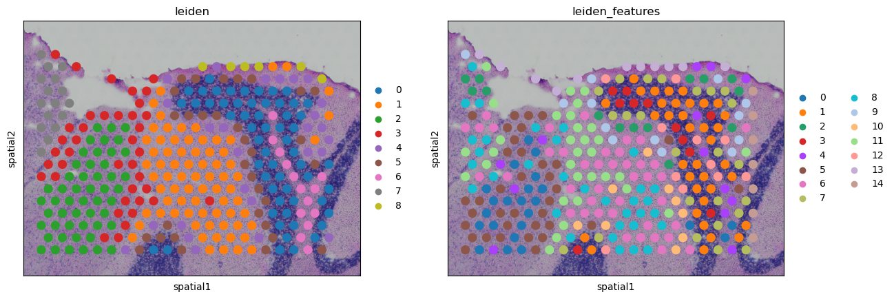
Visualize the result interactively using Napari, or statically using squidpy.pl.spatial_scatter():

.. code-block:: python

img.interactive(adata, library_key=’library_id’)

sq.pl.spatial_scatter(
    adata_crop,
    library_key="library_id",
    crop_coord=(5700, 2700, 9000, 6000),
    library_id=library_ids[0],
    color=["leiden", "leiden_features"],
)

sq.pl.spatial_scatter(
    adata_crop,
    library_key="library_id",
    crop_coord=(5700, 3500, 9000, 6000),
    library_id=library_ids[1],
    color=["leiden", "leiden_features"],
)