%matplotlib inline

Compute Sepal score

This example shows how to compute the Sepal score for spatially variable genes identification.

The Sepal score is a method that simulates a diffusion process to quantify spatial structure in tissue. See [Anderson and Lundeberg, 2021] for reference.

See also

- See {doc}`compute_co_occurrence` and
  {doc}`compute_moran` for other scores to identify spatially variable genes.
- See {doc}`compute_spatial_neighbors` for general usage of
  {func}`squidpy.gr.spatial_neighbors`.

import squidpy as sq

adata = sq.datasets.visium_hne_adata()
adata

AnnData object with n_obs × n_vars = 2688 × 18078
    obs: 'in_tissue', 'array_row', 'array_col', 'n_genes_by_counts', 'log1p_n_genes_by_counts', 'total_counts', 'log1p_total_counts', 'pct_counts_in_top_50_genes', 'pct_counts_in_top_100_genes', 'pct_counts_in_top_200_genes', 'pct_counts_in_top_500_genes', 'total_counts_mt', 'log1p_total_counts_mt', 'pct_counts_mt', 'n_counts', 'leiden', 'cluster'
    var: 'gene_ids', 'feature_types', 'genome', 'mt', 'n_cells_by_counts', 'mean_counts', 'log1p_mean_counts', 'pct_dropout_by_counts', 'total_counts', 'log1p_total_counts', 'n_cells', 'highly_variable', 'highly_variable_rank', 'means', 'variances', 'variances_norm'
    uns: 'cluster_colors', 'hvg', 'leiden', 'leiden_colors', 'neighbors', 'pca', 'rank_genes_groups', 'spatial', 'umap'
    obsm: 'X_pca', 'X_umap', 'spatial'
    varm: 'PCs'
    obsp: 'connectivities', 'distances'

We can compute the Sepal score with squidpy.gr.sepal(). there are 2 important aspects to consider when computing sepal:

• The function only accepts grid-like spatial graphs. Make sure to specify the maximum number of neighbors in your data (6 for an hexagonal grid like Visium) with max_neighs = 6.

• It is useful to filter out genes that are expressed in very few observations and might be wrongly identified as being spatially variable. If you are performing pre-processing with Scanpy, there is a convenient function that can be used BEFORE normalization scanpy.pp.calculate_qc_metrics(). It computes several useful summary statistics on both observation and feature axis. We will be using the n_cells columns in adata.var to filter out genes that are expressed in less than 100 observations.

Before computing the Sepal score, we first need to compute a spatial graph with squidpy.gr.spatial_neighbors(). We will also subset the number of genes to evaluate for efficiency purposes.

sq.gr.spatial_neighbors(adata)
genes = adata.var_names[(adata.var.n_cells > 100) & adata.var.highly_variable][0:100]
sq.gr.sepal(adata, max_neighs=6, genes=genes, n_jobs=1)
adata.uns["sepal_score"].head(10)

	sepal_score
Lct	7.868
1500015O10Rik	7.085
Ecel1	5.274
Fzd5	4.694
Cfap65	4.095
C1ql2	3.144
Slc9a2	2.947
Gm17634	2.904
St18	2.584
Des	2.494

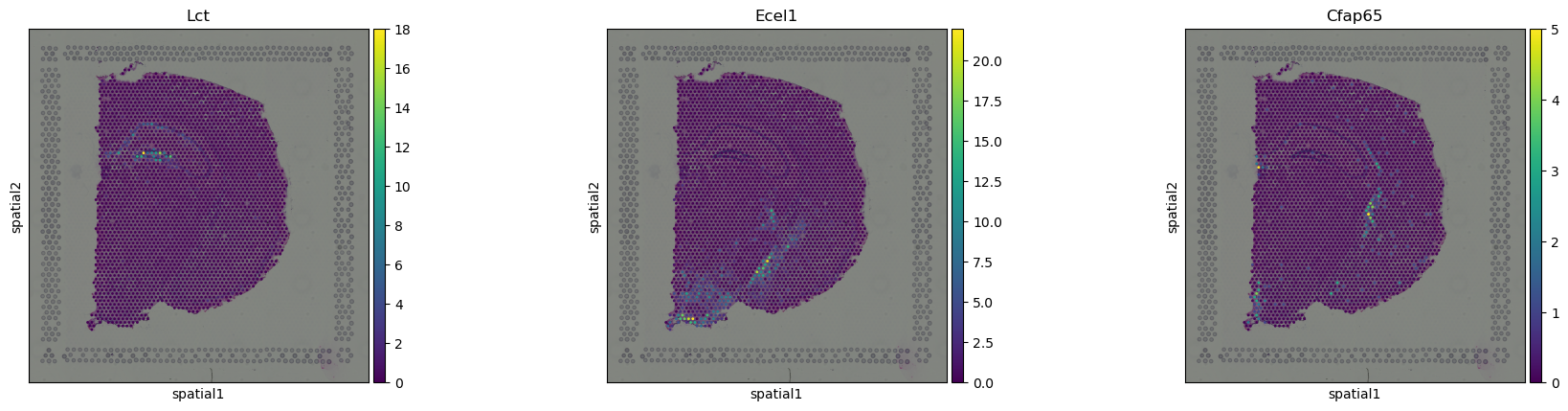
We can visualize some of those genes with squidpy.pl.spatial_scatter().

sq.pl.spatial_scatter(adata, color=["Lct", "Ecel1", "Cfap65"])