%matplotlib inline

Plot scatter plot in spatial coordinates

This example shows how to use squidpy.pl.spatial_scatter to plot annotations and features stored in anndata.AnnData.

This plotting is useful when points and underlying image are available.

See also

See {doc}`plot_segment` for segmentation
masks.

import anndata as ad
import scanpy as sc
import squidpy as sq

adata = sq.datasets.visium_hne_adata()

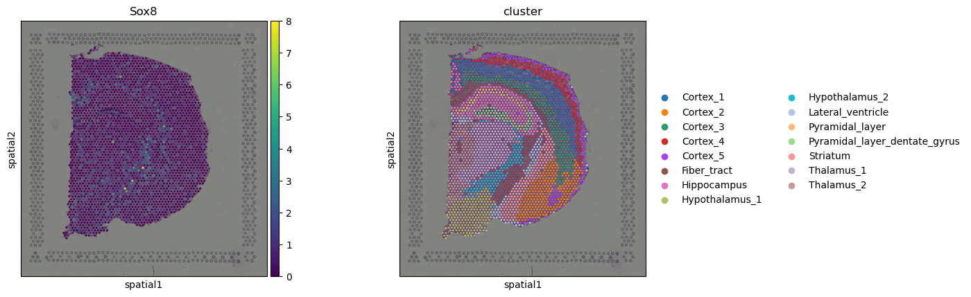
We can take a quick look at the Visium dataset by plotting cluster label and gene expression of choice.

sq.pl.spatial_scatter(adata, color=["Sox8", "cluster"])

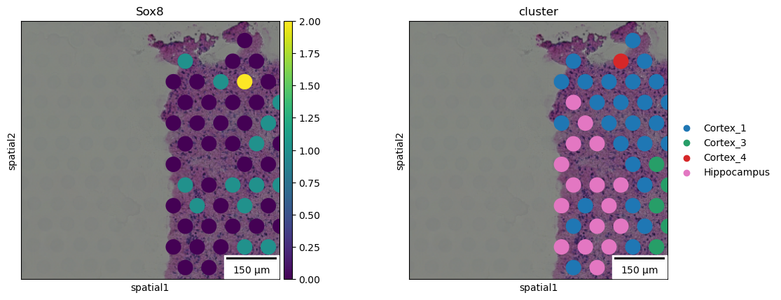
squidpy.pl.spatial_scatter closely resembles scanpy.pl.spatial but it provides additional functionalities. For instance, with the `shape` argument it’s possible to plot polygons such as square or hexagons, a useful feature when technologies other than Visium are used, such as Dbit-seq. Furthermore, it’s also possible to plot a scale bar, where size and pixel units must be passed. The size for this example are not the real values and are for purely visualization purposes.

sq.pl.spatial_scatter(
    adata,
    color=["Sox8", "cluster"],
    crop_coord=[(1500, 1500, 3000, 3000)],
    scalebar_dx=3.0,
    scalebar_kwargs={"scale_loc": "bottom", "location": "lower right"},
)

A key feature of squidpy.pl.spatial_scatter is that it can handle multiple slides datasets. For the purpose of showing this functionality, let’s create a new anndata.AnnData with two Visium slides. We’ll also build the spatial graph, to show the edge plotting functionality.

sq.gr.spatial_neighbors(adata)
adata2 = sc.pp.subsample(adata, fraction=0.5, copy=True)
adata2.uns["spatial"] = {}
adata2.uns["spatial"]["V2_Adult_Mouse_Brain"] = adata.uns["spatial"][
    "V1_Adult_Mouse_Brain"
]
adata_concat = ad.concat(
    {"V1_Adult_Mouse_Brain": adata, "V2_Adult_Mouse_Brain": adata2},
    label="library_id",
    uns_merge="unique",
    pairwise=True,
)
sq.pl.spatial_scatter(
    adata_concat,
    color=["Sox8", "cluster"],
    library_key="library_id",
    connectivity_key="spatial_connectivities",
    edges_width=2,
    crop_coord=[(1500, 1500, 3000, 3000), (1500, 1500, 3000, 3000)],
)

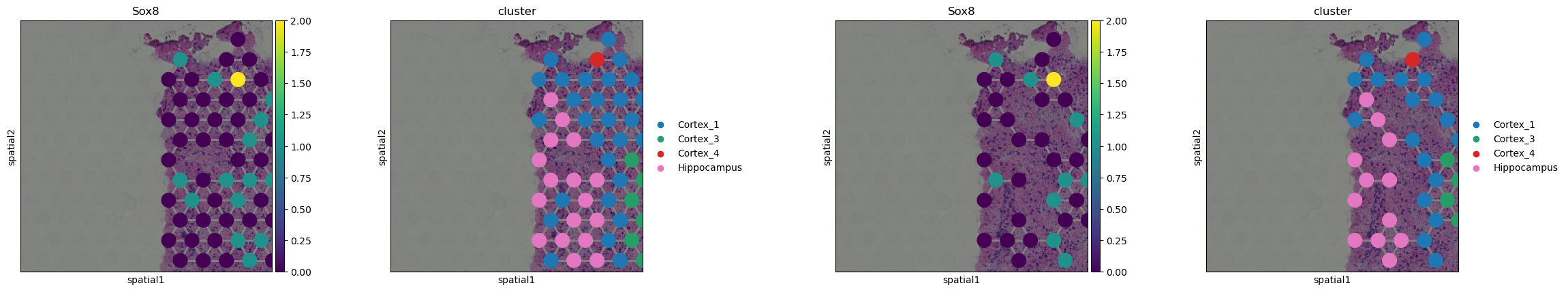
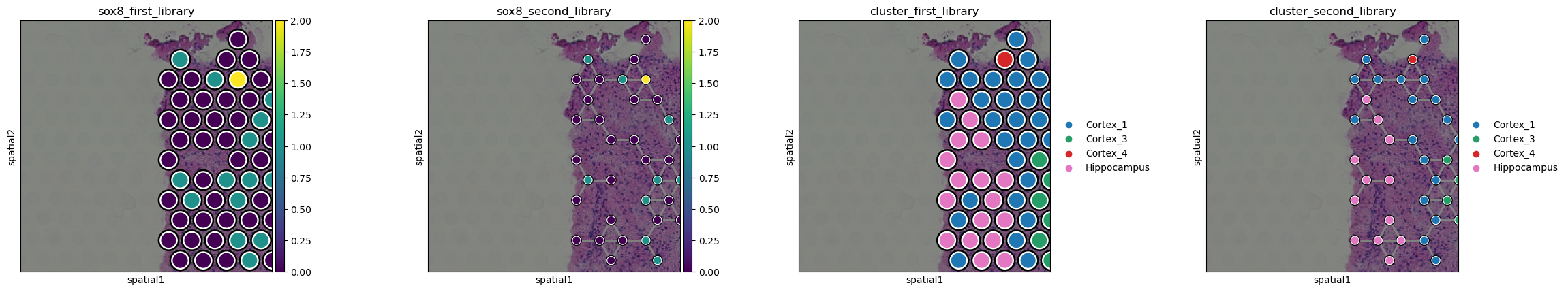
In the above plots, the two Visium datasets are cropped and plotted sequentially. It’s possible to select which plots should be plotted first with the `library_first[ argument. Furthermore, it’s also possible to selectively modify each library, for instance, changing the size of the points as well as the cropping coordinates. To do so, lists can be passed to those arguments, with the same number of elements as the Visium slides to be plotted. This applies to all elements which could be dataset specific, such as ]{.title-ref}title[, ]{.title-ref}outline_width[, ]{.title-ref}size` etc.

sq.pl.spatial_scatter(
    adata_concat,
    color=["Sox8", "cluster"],
    library_key="library_id",
    library_first=False,
    connectivity_key="spatial_connectivities",
    edges_width=2,
    crop_coord=[(1500, 1500, 3000, 3000), (1500, 1500, 3000, 3000)],
    outline=True,
    outline_width=[0.05, 0.05],
    size=[1, 0.5],
    title=[
        "sox8_first_library",
        "sox8_second_library",
        "cluster_first_library",
        "cluster_second_library",
    ],
)

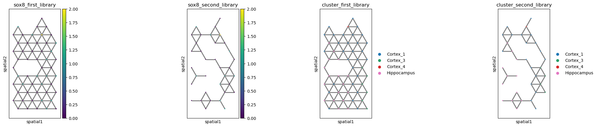
If no image is present, a simple scatter plot will be plotted, but the rest of the functionality remains unchanged. It’s important to specify `shape=None[ in order to default to plain scatter plot. Furthermore, in this setting the ]{.title-ref}size[ argument represents the actual size of the dot, instead of a scaling factor of the diameter as in the previous plot. See {func}`squidpy.pl.spatial_scatter]{.title-ref} for documentation.

sq.pl.spatial_scatter(
    adata_concat,
    shape=None,
    color=["Sox8", "cluster"],
    library_key="library_id",
    library_first=False,
    connectivity_key="spatial_connectivities",
    edges_width=2,
    crop_coord=[(1500, 1500, 3000, 3000), (1500, 1500, 3000, 3000)],
    outline=True,
    outline_width=[0.05, 0.05],
    size=[1, 0.5],
    title=[
        "sox8_first_library",
        "sox8_second_library",
        "cluster_first_library",
        "cluster_second_library",
    ],
)