%matplotlib inline
Matplotlib is building the font cache; this may take a moment.
Compute Moran’s I score
This example shows how to compute the Moran’s I global spatial auto-correlation statistics.
The Moran’s I global spatial auto-correlation statistics evaluates whether features (i.e. genes) shows a pattern that is clustered, dispersed or random in the tissue are under consideration.
See also
See Compute co-occurrence probability and Compute Ripley’s statistics for other scores to describe spatial patterns.
See Building spatial neighbors graph for general usage of
squidpy.gr.spatial_neighbors().
import squidpy as sq

adata = sq.datasets.visium_hne_adata()
adata
/Users/selman/projects/squidpy/docs/notebooks/.venv/lib/python3.12/site-packages/tqdm/auto.py:21: TqdmWarning: IProgress not found. Please update jupyter and ipywidgets. See https://ipywidgets.readthedocs.io/en/stable/user_install.html
  from .autonotebook import tqdm as notebook_tqdm
/Users/selman/projects/squidpy/docs/notebooks/.venv/lib/python3.12/site-packages/docrep/decorators.py:43: SyntaxWarning: 'n_jobs' is not a valid key!
  doc = func(self, args[0].__doc__, *args[1:], **kwargs)
/Users/selman/projects/squidpy/docs/notebooks/.venv/lib/python3.12/site-packages/docrep/decorators.py:43: SyntaxWarning: 'show_progress_bar' is not a valid key!
  doc = func(self, args[0].__doc__, *args[1:], **kwargs)
INFO Downloading visium_hne_adata.h5ad from https://exampledata.scverse.org/squidpy/visium_hne_adata.h5ad
Downloading data from 'https://exampledata.scverse.org/squidpy/visium_hne_adata.h5ad' to file '/Users/selman/projects/squidpy/docs/notebooks/examples/graph/data/anndata/visium_hne_adata.h5ad'.
100%|████████████████████████████████████████| 329M/329M [00:00<00:00, 343GB/s]
AnnData object with n_obs × n_vars = 2688 × 18078
    obs: 'in_tissue', 'array_row', 'array_col', 'n_genes_by_counts', 'log1p_n_genes_by_counts', 'total_counts', 'log1p_total_counts', 'pct_counts_in_top_50_genes', 'pct_counts_in_top_100_genes', 'pct_counts_in_top_200_genes', 'pct_counts_in_top_500_genes', 'total_counts_mt', 'log1p_total_counts_mt', 'pct_counts_mt', 'n_counts', 'leiden', 'cluster'
    var: 'gene_ids', 'feature_types', 'genome', 'mt', 'n_cells_by_counts', 'mean_counts', 'log1p_mean_counts', 'pct_dropout_by_counts', 'total_counts', 'log1p_total_counts', 'n_cells', 'highly_variable', 'highly_variable_rank', 'means', 'variances', 'variances_norm'
    uns: 'cluster_colors', 'hvg', 'leiden', 'leiden_colors', 'neighbors', 'pca', 'rank_genes_groups', 'spatial', 'umap'
    obsm: 'X_pca', 'X_umap', 'spatial'
    varm: 'PCs'
    obsp: 'connectivities', 'distances'
We can compute the Moran’s I score with squidpy.gr.spatial_autocorr
and mode = 'moran'. We first need to compute a spatial graph with
squidpy.gr.spatial_neighbors. We will also subset the number of genes
to evaluate.
genes = adata[:, adata.var.highly_variable].var_names.values[:100]
sq.gr.spatial_neighbors(adata)
sq.gr.spatial_autocorr(
    adata,
    mode="moran",
    genes=genes,
    n_perms=100,
    n_jobs=1,
)
adata.uns["moranI"].head(10)
INFO Creating graph using `None` transform and `1` libraries.
/var/folders/xy/w8sj_5197yg42f3c2txh8gww0000gn/T/ipykernel_97027/3642335017.py:2: FutureWarning: Calling `spatial_neighbors` is deprecated and will be removed in squidpy v1.9.0. Use `spatial_neighbors_knn`, `spatial_neighbors_radius`, `spatial_neighbors_delaunay`, `spatial_neighbors_grid`, or `spatial_neighbors_from_builder` instead.
  sq.gr.spatial_neighbors(adata)
  0%|          | 0/100 [00:00<?, ?/s]/Users/selman/projects/squidpy/docs/notebooks/.venv/lib/python3.12/site-packages/docrep/decorators.py:43: SyntaxWarning: 'n_jobs' is not a valid key!
  doc = func(self, args[0].__doc__, *args[1:], **kwargs)
/Users/selman/projects/squidpy/docs/notebooks/.venv/lib/python3.12/site-packages/docrep/decorators.py:43: SyntaxWarning: 'show_progress_bar' is not a valid key!
  doc = func(self, args[0].__doc__, *args[1:], **kwargs)
100%|██████████| 100/100 [00:23<00:00,  4.34/s]
| I | pval_norm | var_norm | pval_z_sim | pval_sim | var_sim | pval_norm_fdr_bh | pval_z_sim_fdr_bh | pval_sim_fdr_bh | |
|---|---|---|---|---|---|---|---|---|---|
| 3110035E14Rik | 0.665132 | 0.0 | 0.000131 | 0.0 | 0.009901 | 0.000251 | 0.0 | 0.0 | 0.011929 |
| Resp18 | 0.649582 | 0.0 | 0.000131 | 0.0 | 0.009901 | 0.000243 | 0.0 | 0.0 | 0.011929 |
| 1500015O10Rik | 0.605940 | 0.0 | 0.000131 | 0.0 | 0.009901 | 0.000234 | 0.0 | 0.0 | 0.011929 |
| Ecel1 | 0.570304 | 0.0 | 0.000131 | 0.0 | 0.009901 | 0.000255 | 0.0 | 0.0 | 0.011929 |
| 2010300C02Rik | 0.539469 | 0.0 | 0.000131 | 0.0 | 0.009901 | 0.000240 | 0.0 | 0.0 | 0.011929 |
| Scg2 | 0.476060 | 0.0 | 0.000131 | 0.0 | 0.009901 | 0.000164 | 0.0 | 0.0 | 0.011929 |
| Ogfrl1 | 0.457945 | 0.0 | 0.000131 | 0.0 | 0.009901 | 0.000199 | 0.0 | 0.0 | 0.011929 |
| Itm2c | 0.451842 | 0.0 | 0.000131 | 0.0 | 0.009901 | 0.000222 | 0.0 | 0.0 | 0.011929 |
| Tuba4a | 0.451810 | 0.0 | 0.000131 | 0.0 | 0.009901 | 0.000182 | 0.0 | 0.0 | 0.011929 |
| Satb2 | 0.429162 | 0.0 | 0.000131 | 0.0 | 0.009901 | 0.000188 | 0.0 | 0.0 | 0.011929 |
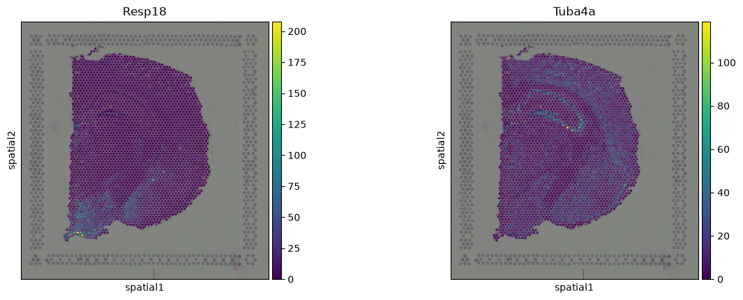
We can visualize some of those genes with squidpy.pl.spatial_scatter.
sq.pl.spatial_scatter(adata, color=["Resp18", "Tuba4a"])
We could’ve also passed mode = 'geary' to compute a closely related
auto-correlation statistic, Geary’s
C. See
squidpy.gr.spatial_autocorr for more information.
Note
Since squidpy 1.8.2, the analytic p-value for Geary’s C (pval_norm) uses the
correct Geary’s C normality variance. Earlier versions reused the Moran’s I
variance, which gave a miscalibrated pval_norm/var_norm for Geary’s C.
Geary’s C analytic p-values therefore differ from earlier versions;
permutation-based p-values are unaffected. See
#1183.